
Scatter Plot Activity
Loading the math board and drawing, please wait…
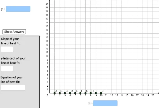
This example demonstrates how to create a scatter plot to visualize data distribution and fit a trend line, involving core concepts like scatter plots, linear regression, slope, and intersection calculations. Key GeoGebra commands used include RemoveUndefined, Segment, FitLineY, Slope, Intersect, and Line, suitable for middle school and above students learning data analysis and geometric constructions.
GeoGebra Commands & Parameters
RemoveUndefined(list3) → list4Corner(2) → H_4Corner(4) → G_4Corner(1) → F_4Segment(F_4, G_4) → hSegment(F_4, H_4) → gTextfield() → InputBox1Textfield() → InputBox2Textfield() → InputBox3Textfield() → InputBox4Polygon(K_4, L_4, I_4, F_4) → poly1, i, j, k, lTextfield() → InputBox5FitLineY(list4) → fSlope(f) → mIntersect(f, yAxis) → E_4Line(K, L) → nIntersect(n, yAxis) → MSlope(n) → m_1If((C2 > 0) ∧ (C3 > 0) ∧ (C4 > 0) ∧ (C5 > 0) ∧ (C6 > 0) ∧ (C7 > 0) ∧ (C8 > 0) ∧ (C9 > 0) ∧ (C10 > 0) ∧ (C11 > 0), true, false) → bIf(C11 > 0, C11 + 2, 25) → yMaxIf(C11 > 0, ((-C11)) / 5, -4) → yMinTextfield(C2) → InputBox6Textfield(C3) → InputBox7Textfield(C4) → InputBox8Textfield(C5) → InputBox9Textfield(C6) → InputBox10Textfield(C7) → InputBox15Textfield(C8) → InputBox11Textfield(C9) → InputBox12Textfield(C10) → InputBox14Textfield(C11) → InputBox13