
Sample Variance Command Demonstration
Loading the math board and drawing, please wait…
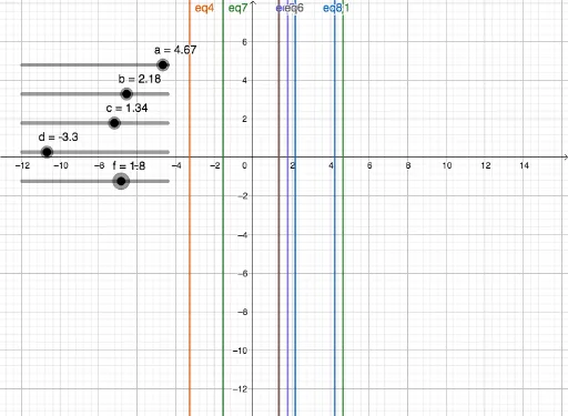
This GeoGebra example demonstrates how to use the SampleVariance command to compute the sample variance of a dataset, along with related statistical measures. The core mathematical concept is descriptive statistics, specifically sample variance, which quantifies the dispersion of data points around the sample mean, calculated as the sum of squared deviations divided by (n-1). The construction uses commands such as mean, Length, Sum, and SampleVariance, involving objects like data lists L1, L2, L3, L4, variables N and SV, and possibly auxiliary elements like histograms and tangent lines. It is suitable for high school or introductory college statistics courses, helping students understand the difference between sample and population variance and how to apply GeoGebra's statistical commands effectively.
GeoGebra Commands & Parameters
mean(L_{1}) → eLength(L_{1}) → NSum(L_{3}) → L_{4}SampleVariance(L_{1}) → g
AI Drawing Prompt Reference
Create a statistical illustration showing sample variance calculation for a dataset. Display a list of data points as a scatter plot or bar chart, with a clear marker for the sample mean. Draw vertical deviation lines from each data point to the mean line to emphasize dispersion. Include a concise formula or numeric result nearby, indicating that sample variance equals the sum of squared deviations divided by the number of data points minus one. Arrange elements clearly to show the relationship between data, mean, deviations, and the final variance value, suitable for classroom demonstration.
The prompt above was compiled from the original drawing commands and is for reference only.