
Roots of an Absolute Value Equation by cemccourseware
Loading the math board and drawing, please wait…
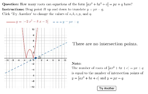
This example demonstrates the graphical representation of the roots of an absolute value equation. Key math concepts include absolute value functions, equation solving, statistical characteristics of roots, linear regression, limits, and logic. Construction highlights involve commands/objects like Random, Element, Expand, RemoveUndefined, Derivative, Intersect, Mirror, Union, Zip, Point, Line, Length, Polygon, Segment, LaTeX, CountIf in GeoGebra. Suitable for high school students learning functions and equations.
GeoGebra Commands & Parameters
Random(-5, 5) → hValRandom(1, 3) → kValElement(lineSlopes, Random[1, 4]) → slopeExpand((aVal * (x - hVal)^(2)) + kVal) → fRemoveUndefined({Intersect[f, xAxis]}) → fRootsDerivative(f) → f'Intersect(f, f'(x) = slope) → TangentPointMirror(TangentPoint, x = hVal) → alternateTangentUnion(fRoots, {Fvertex, TangentPoint, alternateTangent}) → FkeyPtsZip((0, y(A) - (slope * x(A))), A, FkeyPts) → keyYInterceptsUnion(Sequence[(0, i), i, -10, 10, 0.5], keyYIntercepts) → allSliderValsPoint(allSliderVals) → BLine(A, B) → gRemoveUndefined(Union[{Intersect[f, g]}, {Intersect[(-f(x)), g]}]) → allIntersectPtsRemoveUndefined(Zip[If[y(A) ≥ 0, A], A, allIntersectPts]) → positiveIntPtsLength(positiveIntPts) → numIntersectionPtsPolygon({(vbLeft, vbBottom), (vbLeft, vbTop), (vbRight, vbTop), (vbRight, vbBottom)}) → viewboxZip(If[IsInRegion[A, viewbox], true], A, positiveIntPts) → visibleIntPtsSegment((0, floor(vbBottom + 3)), (0, floor(vbTop))) → yAxisVerticalSliderLaTeX(Expand[f]) → LblfLaTeX("\text{\textbf{Note: } \\The number of roots of \(\left\vert ax^2 + bx +c \right\vert =px+q\) \\is equal to the number of intersection points of \\\(y=\left\vert ax^2 + bx + c\right\vert\) and \(y=px+q\).}") → txtNoteCountIf(x ≟ true, visibleIntPts) → numVisibleLaTeX(If[numIntersectionPts ≟ numVisible, "", (("Only " * If[numVisible ≟ 3, "three are", If[numVisible ≟ 2, "two are", "one is"]]) * " visible on the graph.")]) → fbNumVisibleLaTeX(("There " * If[numIntersectionPts ≟ 0, "are no intersection points.", If[numIntersectionPts ≟ 1, "is one intersection point.", (("are " * If[numIntersectionPts ≟ 2, "two", If[numIntersectionPts ≟ 3, "three", "four"]]) * " intersection points. ")]])) → fbNumIntPointsLaTeX((((("\text{" * fbNumIntPoints) * "\\") * fbNumVisible) * "}")) → txtNumIntPtsRemoveUndefined(Zip[If[IsInRegion[A, viewbox], A], A, positiveIntPts]) → allIntersectionsInRegionLaTeX((((("\text{\textbf{Question: }" * MainInstruc) * "\\\textbf{Instructions: }") * SpecInstruc) * "}")) → allInstrucSegment(Element[legendAnchors, 1], Element[legendAnchors, 1] + (3, 0)) → fxLegendSegment(Element[legendAnchors, 2], Element[legendAnchors, 2] + (3, 0)) → lineLegendLaTeX((("\vphantom{\dfrac{1}{2}}y=\left\vert " * Lblf) * " \right\vert")) → lblGraph
AI Drawing Prompt Reference
Draw a graph showing the roots of an absolute value equation, highlighting intersections between an absolute value function and a linear function. Plot the absolute value function and the intersecting line. Mark all intersection points, emphasizing those within the visible range. Calculate and display the total number of intersection points and the number visible in the current view. Add labels for the function expression and explanatory text describing the relationship between intersection points and the roots of the equation.
The prompt above was compiled from the original drawing commands and is for reference only.