
ROC Curve Demonstration
Loading the math board and drawing, please wait…
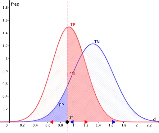
This example demonstrates the construction and visualization of a Receiver Operating Characteristic (ROC) curve. It involves core mathematical concepts such as probability & statistics, curve graphing, and coordinate geometry. Key GeoGebra commands and objects used include Point, Normal, and CurveCartesian. Suitable for high school students and those needing to understand the application of ROC curves in machine learning or statistics.
GeoGebra Commands & Parameters
Point(xAxis) → APoint(xAxis) → A'Normal(A_o, ΔA, x, false) → g_APoint(xAxis) → BPoint(xAxis) → B'Normal(B_o, ΔB, x, false) → g_BPoint(xAxis) → DCurveCartesian((1 - TNR(t), TPR(t)), t, 0, 10) → ROCPoint({1 - P_{TN}, P_{TP}}) → d
AI Drawing Prompt Reference
Draw a ROC curve demonstration, including two vertical lines perpendicular to the x-axis representing normal and abnormal probability points, and a curve connecting these points to show the ROC curve. Mark a point on the curve indicating specific TNR and TPR values.
The prompt above was compiled from the original drawing commands and is for reference only.