
Rigid Body Rotation: Circulation
Loading the math board and drawing, please wait…
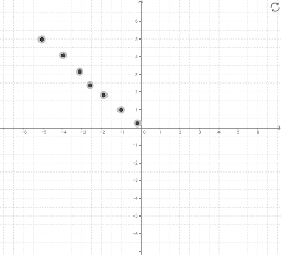
This example demonstrates the flow field of rigid body rotation. Key math concepts include vector fields, velocity distribution, and integral calculations. It is constructed using GeoGebra commands like Textfield, SolveODE, Sequence, SlopeField, Midpoint, SelectedIndex, Element, CurveCartesian, Sum, Segment, Line, etc. Suitable for high school students and math enthusiasts studying rigid body motion and fluid dynamics.
GeoGebra Commands & Parameters
Textfield(x_{min}) → inputBox2Textfield(x_{max}) → inputBox3Textfield(y_{min}) → inputBox4Textfield(y_{max}) → inputBox5SolveODE(f, x(A), y(A), x_{max}, 0.01) → SLVFSolveODE(f, x(A), y(A), x_{min}, 0.01) → SLVBSequence(SolveODE[f, 0, t1, x_{max}, 0.01], t1, -2, 2, 0.25) → SLVFLSequence(SolveODE[f, 0, t1, x_{min}, 0.01], t1, -2, 2, 0.25) → SLVBLSlopeField(f, n, a, x_{min}, y_{min}, x_{max}, y_{max}) → SFSequence(Sequence[Vector[(j, k), (j + (a * v_x(j, k)), k + (a * v_y(j, k)))], j, x_{min}, x_{max}, xstep], k, y_{min}, y_{max}, ystep) → vFieldSolveODE(f, x(B), y(B), x_{max}, 0.01) → numericalIntegral1SolveODE(f, x(C), y(C), x_{max}, 0.01) → numericalIntegral2SolveODE(f, x(D), y(D), x_{max}, 0.01) → numericalIntegral3Midpoint(K, L) → MSelectedIndex(pathNames) → pathIndexElement(pathList, pathIndex) → pathCurveCartesian(x(path(t)), y(path(t)), t, 0, s) → partPathSequence(Vector[path(s), path(s) + ((a * v_x(x(path(s)), y(path(s)))), (a * v_y(x(path(s)), y(path(s)))))], s, 0, 1, 0.1) → pathVectorsSum(Sequence[((path(i + dS) - path(i)) * (v_x(x(path(i + dS / 2)), y(path(i + dS / 2))), v_y(x(path(i + dS / 2)), y(path(i + dS / 2))))), i, 0, s - dS, dS]) → lineIntegralSegment(path(0.2), path(0.21)) → arrow1Segment(path(0.5), path(0.51)) → arrow2Segment(path(0.8), path(0.81)) → arrow3Textfield(time) → InputBox2SolveODE(f, x(F), y(F), x_{max}, 0.01) → numericalIntegral4SolveODE((-y), x, x(E), y(E), x_{max}, 0.01) → numericalIntegral5CurveCartesian((x(E) * cos((w * t))) - (y(E) * sin((w * t))), (x(E) * sin((w * t))) + (y(E) * cos((w * t))), t, 0, time) → stream_1CurveCartesian((x(A) * cos((w * t))) - (y(A) * sin((w * t))), (x(A) * sin((w * t))) + (y(A) * cos((w * t))), t, 0, time) → stream_2CurveCartesian((x(B) * cos((w * t))) - (y(B) * sin((w * t))), (x(B) * sin((w * t))) + (y(B) * cos((w * t))), t, 0, time) → stream_3CurveCartesian((x(C) * cos((w * t))) - (y(C) * sin((w * t))), (x(C) * sin((w * t))) + (y(C) * cos((w * t))), t, 0, time) → stream_4CurveCartesian((x(D) * cos((w * t))) - (y(D) * sin((w * t))), (x(D) * sin((w * t))) + (y(D) * cos((w * t))), t, 0, time) → stream_5CurveCartesian((x(F) * cos((w * t))) - (y(F) * sin((w * t))), (x(F) * sin((w * t))) + (y(F) * cos((w * t))), t, 0, time) → stream_6CurveCartesian((x(Q) * cos((w * t))) - (y(Q) * sin((w * t))), (x(Q) * sin((w * t))) + (y(Q) * cos((w * t))), t, 0, time) → stream_7Line(S, xAxis) → cLine(T, xAxis) → d
AI Drawing Prompt Reference
Draw a flow field diagram for rigid body rotation, showing velocity distribution and integral calculations. Start by plotting direction vectors to represent the velocity field at different points. Then, draw two symmetric curves representing velocity trajectories starting from the minimum and maximum x-values. Add several more curves to show trajectories from different initial points. Finally, include streamlines to depict the motion trajectories over time, and label key areas of the velocity field and paths.
The prompt above was compiled from the original drawing commands and is for reference only.