
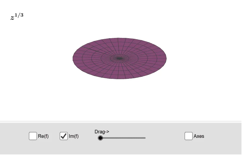
Riemann Surface of z^(1/3)
Loading the math board and drawing, please wait…
This example illustrates the Riemann surface of the cube root of a complex number. It involves complex number power operations and the concept of Riemann surfaces. Users can dynamically adjust parameters to observe the changes of the cube root of a complex number in three-dimensional space. Suitable for high school students and math enthusiasts to learn about complex numbers and Riemann surfaces.
GeoGebra Commands & Parameters
Surface((u * cos(v)), (u * sin(v)), HRe((u * cos(v)), (u * sin(v)), 3, 0), u, 0, 2, v, (-π), π - π / 200) → B0Surface((u * cos(v)), (u * sin(v)), HRe((u * cos(v)), (u * sin(v)), 3, 1), u, 0, 2, v, (-π), π - π / 200) → B1Surface((u * cos(v)), (u * sin(v)), HRe((u * cos(v)), (u * sin(v)), 3, 2), u, 0, 2, v, (-π), π - π / 200) → B2Surface((u * cos(v)), (u * sin(v)), HIm((u * cos(v)), (u * sin(v)), 3, 0), u, 0, 2, v, (-π), π - π / 200) → C0Surface((u * cos(v)), (u * sin(v)), HIm((u * cos(v)), (u * sin(v)), 3, 1), u, 0, 2, v, (-π), π - π / 200) → C1Surface((u * cos(v)), (u * sin(v)), HIm((u * cos(v)), (u * sin(v)), 3, 2), u, 0, 2, v, (-π), π - π / 200) → C2
AI Drawing Prompt Reference
Create a Riemann surface illustrating the cube root of a complex number, featuring three continuous surfaces, each representing the real and imaginary parts of the cube power of a complex number, defined using polar coordinates with parameters u ranging from 0 to 2 and v from -π to π-π/200, showing distinct branches for real and imaginary components, displaying the three-dimensional structure of the complex cube root.
The prompt above was compiled from the original drawing commands and is for reference only.