Riemann Sums: Estimate Area with Interactive Visualization

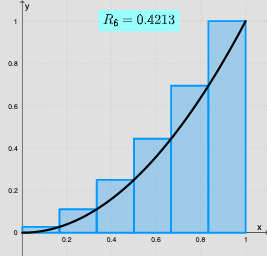
This GeoGebra example dynamically demonstrates how Riemann sums estimate the area under a curve, visually illustrating the process of approximating a definite integral by summing rectangular areas. Core mathematical concepts include definite integrals, Riemann sums (left, right, midpoint, or custom sampling), limits, and area approximation. Construction highlights: The Sequence command generates partition points; Max and Min compute the maximum and minimum function values on each subinterval to create upper (circumscribed) and lower (inscribed) rectangles; Textfield and InputBox provide interactive controls for adjusting the number of subintervals n, the sampling method (e.g., left endpoint, right endpoint, or midpoint), and the function expression; Vector and OrthogonalLine draw rectangle boundaries and vertical lines; If and Sum accumulate the rectangle areas to produce the total estimate. Key objects include the function f, partition list list1, max/min lists maxlist1/minlist1, input boxes InputBox1/2/3, and dynamic texts text1/text2/text3 displaying results. Suitable for high school and college calculus courses, this tool helps students grasp the geometric meaning of integration, compare different Riemann sum types, and observe how estimates converge to the true area as n increases.