Riemann Sum

Loading the math board and drawing, please wait…

2018-11-06 13:54

Function Calculus Integral

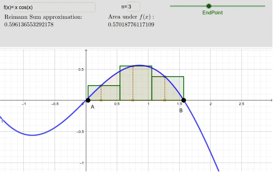
This example demonstrates the geometric interpretation of Riemann sums by dynamically adjusting the number of partitions and intervals, visually showing how Riemann sums approximate the area under a function curve. Key mathematical concepts include integration, continuity, function approximation, and basic calculus. The construction uses GeoGebra commands and objects like Point, Sequence, Textfield, Integral, Sum, focusing on functions, integration, and summation. Suitable for high school students and beginners in calculus learning the geometric intuition of function integration and Riemann sums.

GeoGebra Commands & Parameters

Point(xAxis) → A
Point(xAxis) → B
Sequence(Polygon[Element[Sequence[(x(A) + ((x(B) - x(A)) / n * i), 0), i, 0, n], r], Element[Sequence[(x(A) + ((x(B) - x(A)) / n * i), 0), i, 0, n], r + 1], Element[Sequence[(x(Element[Sequence[(x(A) + ((x(B) - x(A)) / n * i), 0), i, 0, n], j + 1]), y(Element[Sequence[(x(Element[Sequence[(x(A) + ((x(B) - x(A)) / n * i), 0), i, 0, n], k]), f(x(Element[Sequence[(x(A) + ((x(B) - x(A)) / n * i), 0), i, 0, n], k]) + ((x(B) - x(A)) / n * EndPoint))), k, 0, n], j + 1])), j, 1, n], r], Element[Sequence[(x(Element[Sequence[(x(A) + ((x(B) - x(A)) / n * i), 0), i, 0, n], k]), f(x(Element[Sequence[(x(A) + ((x(B) - x(A)) / n * i), 0), i, 0, n], k]) + ((x(B) - x(A)) / n * EndPoint))), k, 0, n], r + 1]], r, 1, n) → Aapprox
Textfield(f) → InputBox1
Textfield(n) → InputBox2
Integral(f, x(A), x(B)) → a
Sum(Aapprox) → b