Riemann Sum Rectangles for Integral Approximation

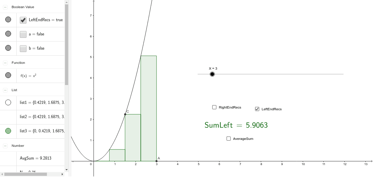
This example demonstrates using Riemann sum rectangles (left, right, and midpoint) to approximate the definite integral, i.e., the area under a curve. By adjusting the number of rectangles N, users can observe how the sum of rectangle areas approaches the actual integral value. Core mathematical concepts include Riemann sums, the definition of definite integrals, and limits. Construction highlights: Sequence command generates equally spaced partition points, Sum command calculates rectangle areas, function f defines the curve, inequalities set integration bounds [a,b], and slider N controls rectangle count. Suitable for high school calculus or college introductory mathematics, helping students intuitively understand integrals as limits.