
Re-parametrization of Vector Functions and Derivatives
Loading the math board and drawing, please wait…
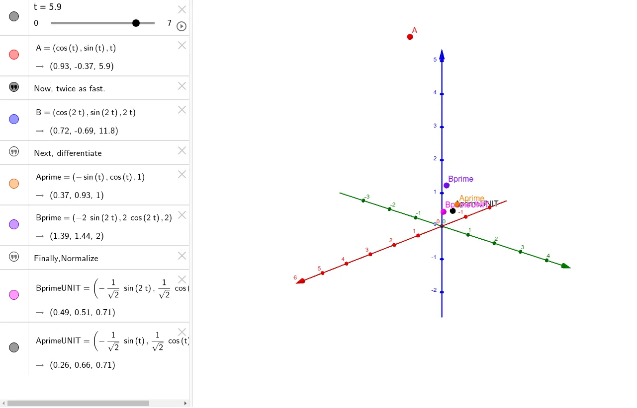
This example demonstrates the graphical transformation of vector functions under different parameterizations and the geometric interpretation of their derivatives. Key math concepts include vector functions, parametric equations, derivatives, and geometric transformations. GeoGebra commands used: t (parameter), A/B (points), text1/text2/text3 (texts), Aprime/Bprime (points), BprimeUNIT/AprimeUNIT (unit vectors). Suitable for university students and teachers in mathematics, physics, and related fields for instructional demonstration and conceptual understanding.
GeoGebra Commands & Parameters
Numeric t(5.9)(cos(t), sin(t), t)(cos((2 * t)), sin((2 * t)), (2 * t))((-sin(t)), cos(t), 1)((-2 * sin((2 * t))), (2 * cos((2 * t))), 2)((-1 / sqrt(2) * sin((2 * t))), (1 / sqrt(2) * cos((2 * t))), 1 / sqrt(2))((-1 / sqrt(2) * sin(t)), (1 / sqrt(2) * cos(t)), 1 / sqrt(2))
AI Drawing Prompt Reference
Draw a vector function graph to demonstrate the geometric interpretation of derivatives under different parameterizations. Start with the curve (cos(t), sin(t), t) for parameter t, then the curve (cos(2t), sin(2t), 2t) for parameter 2t, followed by the curve (-cos(t), sin(t), 1) for parameter -t, the curve (-cos(2t), 2sin(2t), 2) for parameter -2t, the curve (-sin(2t)/√2, cos(2t)/√2, 1/√2) for parameter (2t), and finally the curve (-sin(t)/√2, cos(t)/√2, 1/√2) for parameter t.
The prompt above was compiled from the original drawing commands and is for reference only.