
Rational Function End Behavior
Loading the math board and drawing, please wait…
In collections
AP Calculus AB Applet Collection
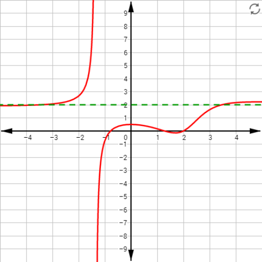
This example demonstrates the end behavior of rational functions. It involves concepts such as the degree of a rational function and asymptotes. Using GeoGebra commands like Simplify and Asymptote, the graph of a rational function can be constructed and its end behavior observed. Suitable for high school mathematics education and learning.
GeoGebra Commands & Parameters
Simplify((NumLC * x^(NumDeg)) + If[NumDeg > 3, ((Random[0, 10] - 5) * x^(3)), 0] + If[NumDeg > 2, ((Random[0, 10] - 5) * x^(2)), 0] + If[NumDeg > 1, Random[0, 10] - 5, 0] + If[NumDeg > 0, Random[0, 10] - 5, 0]) → numSimplify((DenLC * x^(DenDeg)) + If[DenDeg > 3, ((Random[0, 10] - 5) * x^(3)), 0] + If[DenDeg > 2, ((Random[0, 10] - 5) * x^(2)), 0] + If[DenDeg > 1, Random[0, 10] - 5, 0] + If[DenDeg > 0, Random[0, 10] - 5, 0]) → denAsymptote(ratfun) → asymlistElement(asymlist, 1) → HAOAIf(NumDeg > DenDeg, (4 * 10^(Zoom)), 10) → yzoomPosIf(NumDeg > DenDeg, (-4 * 10^(Zoom)), -10) → yzoomNeg
AI Drawing Prompt Reference
Draw the graph of a rational function to demonstrate its end behavior, including horizontal asymptotes and the function's expression, constructed with randomly generated polynomial coefficients, and set appropriate coordinate ranges to observe the function's trends at positive and negative infinity.
The prompt above was compiled from the original drawing commands and is for reference only.