
Quadratic Polynomial Graph
Loading the math board and drawing, please wait…
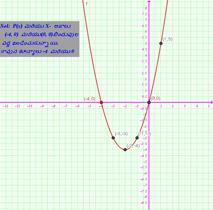
This example demonstrates the graphical representation of a quadratic polynomial. It involves the core mathematical concept of quadratic polynomial functions. Using GeoGebra commands such as Intersect, Sum, and TableText, dynamic observations of the properties of quadratic polynomials can be made. Suitable for high school mathematics education and learning.
GeoGebra Commands & Parameters
Intersect(f(x), y = 0) → A, BSum(B3:D3) → E3Sum(B4:D4) → E4Sum(B5:D5) → E5Sum(B6:D6) → E6Sum(B7:D7) → E7Sum(B8:D8) → E8Sum(B9:D9) → E9Sum(B10:D10) → E10TableText({{A2, B2, C2, D2, E2, F2}, {A3, B3, C3, D3, E3, F3}, {A4, B4, C4, D4, E4, F4}, {A5, B5, C5, D5, E5, F5}, {A6, B6, C6, D6, E6, F6}, {A7, B7, C7, D7, E7, F7}, {A8, B8, C8, D8, E8, F8}, {A9, B9, C9, D9, E9, F9}, {A10, B10, C10, D10, E10, F10}}, "c_|h") → text2Name(B2) → G1
AI Drawing Prompt Reference
Draw the graph of a quadratic polynomial curve, marking its two intersection points with the horizontal axis. Next to the graph, create a table with multiple rows, each containing six numeric values, where the last column is the sum of the first three values. Display a single numeric label near the table, representing the second value from one of the rows. The overall layout should clearly show the curve, the intersection points, and the numeric table for observing properties of the quadratic function.
The prompt above was compiled from the original drawing commands and is for reference only.