
QQ Plots
Loading the math board and drawing, please wait…
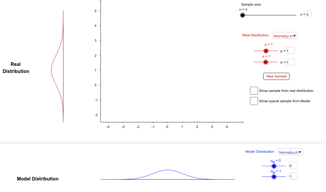
This example demonstrates QQ plots, a graphical method for comparing the distributions of two data sets. Key mathematical concepts include normal, gamma, and exponential distributions in probability and statistics. Using GeoGebra commands such as RandomUniform, Sort, and Mirror, QQ plots are constructed to visually compare different data distributions. Suitable for high school students and statistics enthusiasts.
GeoGebra Commands & Parameters
SelectedIndex(distributionsmodel) → SelectedModelSelectedIndex(distributionsreal) → SelectedRealRandomUniform(0, 1, n) → samplerealZip((-9, InverseNormal[μ, σ, yy]), yy, samplereal) → pointsrealNormalZip((-9, InverseGamma[3, β, yy] - 2), yy, samplereal) → pointsrealGammaZip((-9, InverseExponential[λ, yy] - 2), yy, samplereal) → pointsrealExpZip((-9, InverseGamma[s / 2, 2, yy]), yy, samplereal) → pointsreal2Zip((-9, ((-yy) + s) / sqrt((2 * s)) + 2.5), yy, y(pointsreal2)) → pointsrealSkewLeftZip((-9, (yy - s) / sqrt((2 * s))), yy, y(pointsreal2)) → pointsrealSkewRightIf(SelectedReal ≟ 1, pointsrealNormal, If[SelectedReal ≟ 2, pointsrealExp, If[SelectedReal ≟ 3, pointsrealGamma, If[SelectedReal ≟ 4, pointsrealSkewRight, pointsrealSkewLeft]]]) → pointsRealSort(y(pointsReal)) → ysortRealSequence(k / (n + 1), k, 1, n, 1) → pointsZip((InverseNormal[μ_M, σ_M, yy] - 3, 2.2), yy, points) → pointsmodelNormZip((InverseGamma[3, β_M, yy] - 7, 2.2), yy, points) → pointsmodelGammaZip((InverseExponential[λ_M, yy] - 7, 2.2), yy, points) → pointsmodelExpZip((InverseGamma[s_M / 2, 2, yy], 2.2), yy, points) → pointsmodel2Zip(((yy - s_M) / sqrt((2 * s_M)) - 3, 2.2), yy, x(pointsmodel2)) → pointsmodelSkewRightMirror(pointsmodelSkewRight, x = -3) → pointsmodelSkewLeftIf(SelectedModel ≟ 1, pointsmodelNorm, If[SelectedModel ≟ 2, pointsmodelExp, If[SelectedModel ≟ 3, pointsmodelGamma, If[SelectedModel ≟ 4, pointsmodelSkewRight, pointsmodelSkewLeft]]]) → pointsModelSort(x(pointsModel)) → xsortModelIf(SelectedReal ≟ 1, pointsrealNormal, If[SelectedReal ≟ 2, pointsrealExp, If[SelectedReal ≟ 3, pointsrealGamma, If[SelectedReal ≟ 4, pointsrealSkewRight, pointsrealSkewLeft]]]) → points1Sort(y(points1)) → points3Zip((InverseExponential[λ_M, yy] - 7, xx), yy, points, xx, points3) → FexpZip((InverseGamma[3, β_M, yy] - 7, xx), yy, points, xx, points3) → FgammaZip((x(xx), yy), xx, pointsModel, yy, points3) → FSkewRightZip((x(xx), yy), xx, pointsModel, yy, points3) → FSkewLeftauxZip((xx, yy), xx, xsortModel, yy, ysortReal) → FSkewLeftZip((InverseNormal[μ_M, σ_M, yy] - 3, xx), yy, points, xx, points3) → FnormGamma(s_M / 2, 2, x) → g_MGamma(s / 2, 2, x) → gGamma(3, β_M, x) → GammaModelNormal(μ_M, σ_M, x) → NormalModelExponential(λ_M, x) → ExpModelGamma(3, β, x) → GammaRealExponential(λ, x) → ExpRealNormal(μ, σ, x) → NormalRealIf(SelectedReal ≟ 1, σ, If[SelectedReal ≟ 2, 1 / λ^(2), 3 / β^(2)]) → varRealIf(SelectedReal ≟ 1, μ, If[SelectedReal ≟ 2, 1 / λ, 3 / β]) → meanRealElement(rulesreal, SelectedReal) → frealSort(samplereal) → samplerealordElement(rulesmodel, SelectedModel) → fmodelQ1(xpointsModel) → q1ModelQ3(xpointsModel) → q3ModelIf(SelectedModel ≟ 1, μ_M, If[SelectedModel ≟ 2, 1 / λ_M, 3 / β_M]) → meanModelIf(SelectedModel ≟ 1, σ_M, If[SelectedModel ≟ 2, 1 / λ_M^(2), 3 / β_M^(2)]) → varModelMax(x(pointsModel)) → xMaxpointsModelTranslate(Rotate[frealrestrict, 1.5708], (-10, 0)) → gNormSkewSegment((-10, -2.5), (-10, 5)) → RealpdfAxisSegment((-9, -2.5), (-9, 5)) → RealsampleAxisSequence(Text[i, (-7.9, i - 0.1)], i, -2, 5) → listyyNormSkewRightSequence(Text[i, (i - 3.1, -2.9)], i, -4, 4) → listxxNormSkewSequence(Text[i, (-7.9, i - 2.1)], i, 0, 7) → listyyExpGammaTranslate(Rotate[frealrestrict, 1.5708], (-10, -2)) → gExpGammaSegment((-7.5, 2.2), (1.5, 2.2)) → modelaxisIf(SelectedModel ≟ 1, Fnorm, If[SelectedModel ≟ 2, Fexp, If[SelectedModel ≟ 3, Fgamma, If[SelectedModel ≟ 4, FSkewRight, FSkewLeft]]]) → QQpointsElement(QQpoints, 2) → Min2QQElement(pointsModel, 2) → Min2ModelElement(pointsModel, n - 1) → MaxModelPolygon((x(Corner[1]) + 4.5, y(Corner[1]) + 0.8), (x(Corner[1]), y(Corner[1]) + 0.8), (x(Corner[1]), y(Corner[1])), (x(Corner[1]) + 4.5, y(Corner[1]))) → bottombar, k, l, m, pSegment(Min2Real, Min2QQ) → ASegment(Min2QQ, (x(Min2QQ), -4)) → DPolygon((x(Corner[4]), y(Corner[4])), (x(Corner[4]) + 4.6, y(Corner[4])), (x(Corner[4]) + 4.6, y(Corner[4]) - 0.7), (x(Corner[4]), y(Corner[4]) - 0.7)) → topbar, a_1, c, d, eNormal(0, 1, x) → SnormPolygon((x(Corner[2]) - 5.5, y(Corner[2])), Corner[2], Corner[3] + 1, (x(Corner[3]) - 5.5, y(Corner[3]) + 1)) → sidebar, a, f, h, iGamma(s / 2, 0.5, sqrt((2 * s)) + s) → bZip(InverseGamma[s / 2, 2, yy], yy, samplereal) → SkewpointsSequence(Text[i, (i - 7.1, -2.9)], i, 0, 8) → listxxExpGammaSegment((-7.5, 0), (1.5, 0)) → xaxisbottomSequence(Segment[Element[pointsModel, i], (x(Element[pointsModel, i]), 0)], i, 1, n) → LinesModelElement(QQpoints, n - 1) → Max2QQSegment(Max2Real, Max2QQ) → BSegment(Max2QQ, (x(Max2QQ), -4)) → ESegment((x(MaxModel), 3), (x(MaxModel), 2.2)) → LSegment((x(Min2Model), 3), (x(Min2Model), 2.2)) → JSequence(Text[i, (-7.9, i + 3 - 0.1)], i, -5, 2) → listyySkewLeftFractionText(1 / (n + 1)) → fraction1FractionText(1 / (n + 1)) → fraction2Textfield(μ) → μInputTextfield(σ) → σInputTextfield(λ) → λInputTextfield(β) → βInputTextfield(s) → sInputTextfield(μ_M) → μ_mInputTextfield(σ_M) → σ_MInputTextfield(λ_M) → λ_mInputTextfield(β_M) → β_mInputTextfield(s_M) → s_mInputPolygon((x(Corner[2]) - 5.5, y(Corner[2])), Corner[2], Corner[3] + 1, (x(Corner[3]) - 5.5, y(Corner[3]) + 1)) → sidebar2, j, q, r, tTextfield(n) → nInput
AI Drawing Prompt Reference
Draw a QQ plot (Quantile-Quantile Plot) to compare two datasets' distributions. The first dataset is generated from random numbers and follows distributions such as normal, gamma, or exponential. The second dataset is the theoretical cumulative distribution function of these distributions. The QQ plot compares data quantiles with theoretical quantiles, showing the similarity between data and theoretical distributions. Construct it by generating random samples, computing quantiles and their cumulative probabilities, and plotting the comparison.
The prompt above was compiled from the original drawing commands and is for reference only.