
Pythagoras' Theorem Part 6
Loading the math board and drawing, please wait…
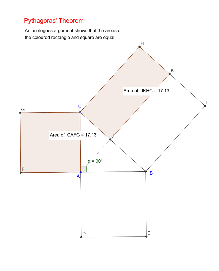
This example demonstrates the 6th part of Pythagoras' theorem, showing the relationship between the hypotenuse and the legs of a right triangle. Key mathematical concepts include the properties of right triangles and similarity transformations. Using GeoGebra commands such as Segment, OrthogonalLine, and Point, a dynamic geometric model is constructed. Suitable for middle school and above students to explore geometric transformations and Pythagoras' theorem.
GeoGebra Commands & Parameters
Segment(A, B) → aOrthogonalLine(A, a) → bPoint(b) → CSegment(C, A) → cSegment(C, B) → dAngle(B, A, C) → αCircle(B, A) → eCircle(A, B) → fOrthogonalLine(B, a) → gOrthogonalLine(A, a) → hIntersect(f, h, 1) → DIntersect(e, g, 1) → ESegment(D, E) → iSegment(B, A) → jSegment(A, D) → kSegment(E, B) → lCircle(A, C) → pCircle(C, A) → qOrthogonalLine(A, c) → mIntersect(p, m, 1) → FOrthogonalLine(C, c) → nIntersect(q, n, 1) → GOrthogonalLine(C, d) → rOrthogonalLine(B, d) → sCircle(B, C) → tCircle(C, B) → c_1Intersect(c_1, r, 2) → HIntersect(t, s, 2) → ISegment(B, I) → a_1Segment(I, H) → b_1Segment(H, C) → d_1Segment(C, G) → e_1Segment(F, A) → f_1Segment(F, G) → g_1OrthogonalLine(A, d) → h_1Intersect(h_1, d) → JIntersect(h_1, b_1) → KSegment(A, J) → i_1Polygon(J, K, H, C) → poly1, j_1, k_1, h_2, c_2Polygon(C, A, F, G) → poly2, c_3, a_2, f_2, g_2PointIn(poly1) → Pointpoly1PointIn(poly2) → Pointpoly2
AI Drawing Prompt Reference
Draw a right triangle ABC with AB as the hypotenuse and AC and BC as the legs. Construct the altitude from C to AB, and use it to draw other lines and circles based on the properties of right triangles and similarity transformations. Finally, form two quadrilaterals and two triangles to explore Pythagoras' theorem.
The prompt above was compiled from the original drawing commands and is for reference only.