Properties of Gradient Vector Field (2014) – Directional Derivative on Unit Circ

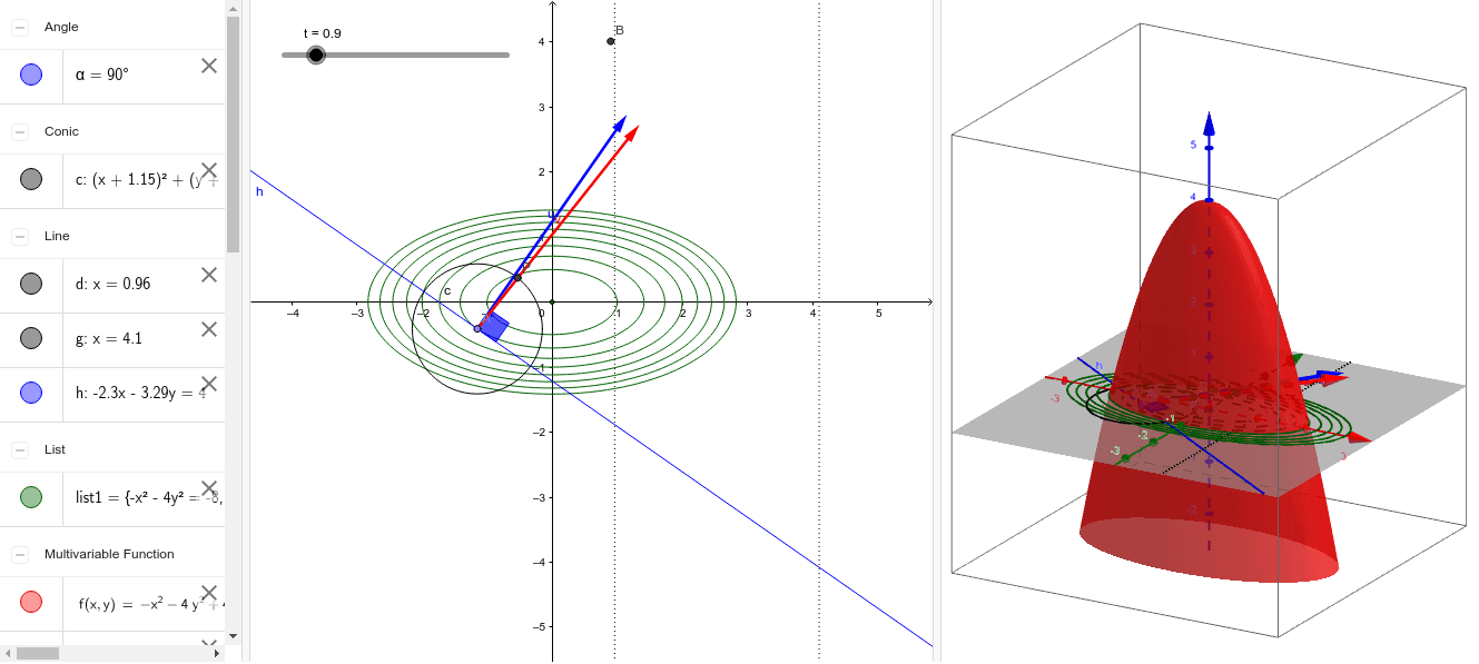
① This example demonstrates the geometric meaning of the directional derivative in a gradient vector field by moving a point on the unit circle to explore how the rate of change varies with direction. ② Core mathematical concepts include gradient vectors, directional derivatives, partial derivatives, and vector fields, fundamental to multivariable calculus. ③ Construction highlights: using GeoGebra commands such as Sequence, Derivative, Point, Vector, Circle, OrthogonalLine, Intersect, and Angle, the applet builds a function f, its partial derivatives f_x and f_y, a direction vector u controlled by a point A on the unit circle, and auxiliary lines/points to visualize the projection of the gradient onto the direction. ④ Suitable for university-level calculus or advanced high school students, ideal for classroom demonstrations to foster intuitive understanding of directional derivatives and gradient properties.