
Projections of a Spherical Trochoid: Parametric Curves via 3D Geometry
Loading the math board and drawing, please wait…
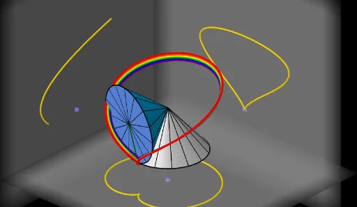
This example demonstrates how a spherical trochoid’s shape changes when projected onto different planes, producing distinct parametric curve traces. The mathematical ideas include spherical curves (spherical trochoids), projections from 3D geometric setups onto planes, and the way parameter-driven motion generates locus-like tracks. Construction-wise, it first builds a Sphere as the underlying surface, then uses Circle and Cone to define the rolling/rotational geometric structure. A Plane and suitable projection Lines establish where the projection is taken. The resulting projected curve is then generated as a Cartesian parametric curve using CurveCartesian, while key orientation constraints are handled through Angle and AngularBisector. Points along the motion are generated via Sequence/Point objects to sample the parameter t, and segments/surfaces are used to visualize the spatial configuration. GeoGebra commands and key objects include CurveCartesian, Sphere, Circle, Cone, Plane, Surface, Line, Segment, Angle, AngularBisector, Sequence, and Point, together with parameters like t/speed and geometric constants (e.g., radii and reference points) to drive the animation. Suitable for secondary-to-university learners studying solid geometry, loci/trajectories, and parametric curve visualization.
GeoGebra Commands & Parameters
CurveCartesian(((a - (b * cos(w)) + (((b + d) * cos(w)) * cos((a / b * t)))) * cos(t)) + (((b + d) * sin(t)) * sin((a / b * t))), ((a - (b * cos(w)) + (((b + d) * cos(w)) * cos((a / b * t)))) * sin(t)) - (((b + d) * cos(t)) * sin((a / b * t))), (sin(w) * (b - ((b + d) * cos((a / b * t))))), t, 0, ((2 * π) * b)) → eSphere((0, 0, h), R) → cCircle((0, 0, 0), a, zAxis) → fCone(C, O, b) → g, k, iCone((0, 0, 0), O, a) → j, p, lSegment(O, E_t) → mAngle(O + (0, 0, -1), O, (a, 0, 0)) → αSegment(O, (a, 0, 0)) → rSurface(((r * cos(u)) * cos(v)), ((r * sin(u)) * cos(v)), h + (r * sin(v)), u, 0, 6.28319, v, -1.5708, ((-π)) / 2 + α) → hsSegment(C, E_t) → qSequence(Rotate[r, i, zAxis], i, 0, 6.28319, ((2 * π / n) * b / a)) → liste1CurveCartesian(((a - (b * cos(w)) + (((b + d) * cos(w)) * cos((a / b * t)))) * cos(t)) + (((b + d) * sin(t)) * sin((a / b * t))), ((a - (b * cos(w)) + (((b + d) * cos(w)) * cos((a / b * t)))) * sin(t)) - (((b + d) * cos(t)) * sin((a / b * t))), (sin(w) * (b - ((b + d) * cos((a / b * t))))), t, 0, tt) → oSequence(Segment[Rotate[C, i, Line[C, O]], Rotate[E_0, i, Line[C, O]]], i, 0, 6.28319, (2 * π / n)) → liste3Sequence(Segment[Rotate[O, i, Line[O, C]], Rotate[E_0, i, Line[O, C]]], i, 0, 6.28319, (2 * π / n)) → liste2Circle(C, b, Line[C, O]) → cmCurveCartesian(((a - (b * cos(w)) + (((b - 0.25) * cos(w)) * cos((a / b * t)))) * cos(t)) + (((b - 0.25) * sin(t)) * sin((a / b * t))), ((a - (b * cos(w)) + (((b - 0.25) * cos(w)) * cos((a / b * t)))) * sin(t)) - (((b - 0.25) * cos(t)) * sin((a / b * t))), (sin(w) * (b - ((b - 0.25) * cos((a / b * t))))), t, 0, tt) → tCurveCartesian(((a - (b * cos(w)) + (((b - 0.5) * cos(w)) * cos((a / b * t)))) * cos(t)) + (((b - 0.5) * sin(t)) * sin((a / b * t))), ((a - (b * cos(w)) + (((b - 0.5) * cos(w)) * cos((a / b * t)))) * sin(t)) - (((b - 0.5) * cos(t)) * sin((a / b * t))), (sin(w) * (b - ((b - 0.5) * cos((a / b * t))))), t, 0, tt) → uCurveCartesian(((a - (b * cos(w)) + (((b - 0.75) * cos(w)) * cos((a / b * t)))) * cos(t)) + (((b - 0.75) * sin(t)) * sin((a / b * t))), ((a - (b * cos(w)) + (((b - 0.75) * cos(w)) * cos((a / b * t)))) * sin(t)) - (((b - 0.75) * cos(t)) * sin((a / b * t))), (sin(w) * (b - ((b - 0.75) * cos((a / b * t))))), t, 0, tt) → vCurveCartesian(((a - (b * cos(w)) + (((b - 1) * cos(w)) * cos((a / b * t)))) * cos(t)) + (((b - 1) * sin(t)) * sin((a / b * t))), ((a - (b * cos(w)) + (((b - 1) * cos(w)) * cos((a / b * t)))) * sin(t)) - (((b - 1) * cos(t)) * sin((a / b * t))), (sin(w) * (b - ((b - 1) * cos((a / b * t))))), t, 0, tt) → a_1CurveCartesian(((a - (b * cos(w)) + (((b - 1.25) * cos(w)) * cos((a / b * t)))) * cos(t)) + (((b - 1.25) * sin(t)) * sin((a / b * t))), ((a - (b * cos(w)) + (((b - 1.25) * cos(w)) * cos((a / b * t)))) * sin(t)) - (((b - 1.25) * cos(t)) * sin((a / b * t))), (sin(w) * (b - ((b - 1.25) * cos((a / b * t))))), t, 0, tt) → b_1Point(zAxis) → DPoint(xAxis) → BAngularBisector(yAxis, xAxis) → g_1, h_1Line(B, h_1) → i_1Line(B, zAxis) → f_1Point(i_1) → EPoint(f_1) → FPlane(B, E, F) → q_1CurveCartesian(x(B), y(B) + (a * cos(i)^(2)), z(B) + ((a^(2) * cos(i)^(3)) * sin(i) / b), i, 0, tt) → d_1CurveCartesian(x(D) + ((a - (b * cos(w)) + (((b + d) * cos(w)) * cos((a / b * t)))) * cos(t)) + (((b + d) * sin(t)) * sin((a / b * t))), y(D) + ((a - (b * cos(w)) + (((b + d) * cos(w)) * cos((a / b * t)))) * sin(t)) - (((b + d) * cos(t)) * sin((a / b * t))), z(D) + ((0 * sin(w)) * (b - ((b + d) * cos((a / b * t))))), t, 0, tt) → c_1CurveCartesian(x(B) + ((0 * (a - (b * cos(w)) + (((0 * (b + d)) * cos(w)) * cos((a / b * t))))) * cos(t)) + (((0 * (b + d)) * sin(t)) * sin((a / b * t))), y(B) + ((a - (b * cos(w)) + (((b + d) * cos(w)) * cos((a / b * t)))) * sin(t)) - (((b + d) * cos(t)) * sin((a / b * t))), z(B) + (sin(w) * (b - ((b + d) * cos((a / b * t))))), t, 0, tt) → e_1Line(B, yAxis) → j_1Line(B, zAxis) → k_1Point(j_1) → GPoint(k_1) → HPlane(G, B, H) → r_1Point(yAxis) → ICurveCartesian(x(I) + ((a - (b * cos(w)) + (((b + d) * cos(w)) * cos((a / b * t)))) * cos(t)) + (((b + d) * sin(t)) * sin((a / b * t))), y(I), z(I) + (sin(w) * (b - ((b + d) * cos((a / b * t))))), t, 0, tt) → l_1Line(I, xAxis) → m_1Line(I, zAxis) → n_1Point(m_1) → JPoint(n_1) → KPlane(J, I, K) → p_2
AI Drawing Prompt Reference
Visualize the projection of a spherical trochoid onto different planes, showing how its shape changes. Start by constructing a sphere as the base surface, then build a circle and a cone to define the rolling/rotational structure. Use planes and projection lines to establish where the projections occur. Generate the projected curves using parametric equations. Sample points along the motion to visualize the parameter-driven trajectory, and use segments and surfaces to illustrate the spatial configuration.
The prompt above was compiled from the original drawing commands and is for reference only.