
Viviani Curve: a Parametric Trajectory from Sphere–Cone (or Cylinder) Intersecti
Loading the math board and drawing, please wait…
In collections
intersection: surface-surface, curve-curve
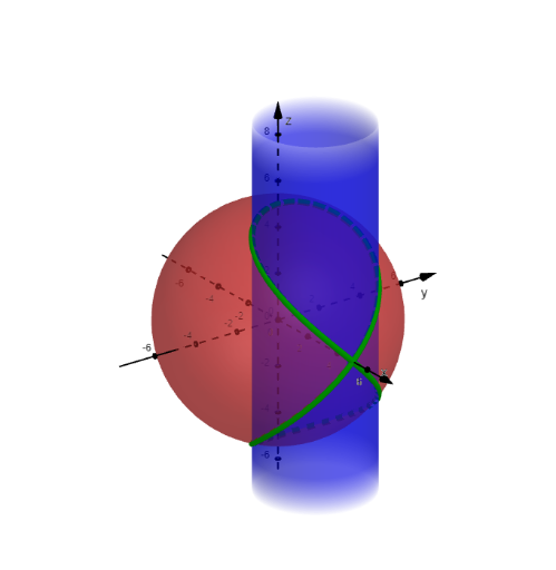
This example demonstrates how the Viviani curve arises as an intersection (a spatial locus) obtained by cutting a sphere with a cone/cylinder-like solid. The key ideas are parametric/Cartesian curve construction, 3D solid geometry, and the geometric meaning of an intersection curve (Schnittkurve) that becomes a well-known trajectory. The construction uses GeoGebra commands such as CurveCartesian to define the curve r in Cartesian coordinates, creates solids via Kugel (sphere) and Zylinder (cylinder), introduces coordinate parameters like x1, x2, x3 to control the configuration, and finally applies Schnittkurve to compute and visualize the intersection curve. Suitable for secondary-school advanced geometry, and introductory college topics in analytic/solid geometry and locus/parametric curves.
GeoGebra Commands & Parameters
CurveCartesian(x1(t), x2(t), x3(t), t, 0, (6 * pi)) → Schnittkurve
AI Drawing Prompt Reference
Draw a three-dimensional Viviani curve, which is the spatial intersection of a sphere and a cylinder. First construct a sphere, then place a cylinder with its axis passing through the sphere's center and tilted so that it cuts through the sphere. Highlight the resulting intersection curve, a closed, spiral-like path that winds on the sphere's surface. The curve can be defined parametrically over a full period. Show both solids as semi-transparent surfaces to clearly reveal their intersection.
The prompt above was compiled from the original drawing commands and is for reference only.