
Projectile Motion Visualization
Loading the math board and drawing, please wait…
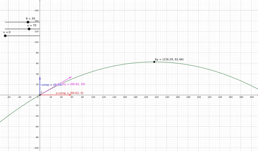
This example demonstrates the trajectory and dynamic changes of projectile motion. It involves core mathematical concepts such as vectors, 2D coordinates, angles, quadratic functions, parabolas, and coordinate geometry. Constructed using GeoGebra commands like Vector, Angle, displacement, time, and velocity. Suitable for high school physics and mathematics teaching to understand kinematics principles and the relationship between function graphs and motion.
GeoGebra Commands & Parameters
Vector((a, f(a)), (a + (u * cos(θ°)), f(a) + (((1 - ((2 * a)) / x(Δx)) * u) * sin(θ°)))) → sVector((a, f(a)), (a + (u * cos(θ°)), f(a))) → vVector((a, f(a)), (a, f(a) + (((1 - ((2 * a)) / x(Δx)) * u) * sin(θ°)))) → w
AI Drawing Prompt Reference
Visualize a projectile motion trajectory in a 2D coordinate system, showing the path of an object with initial velocity vector, horizontal and vertical velocity vectors, and marking key points like the start, peak, and landing positions. Use a parabolic function to represent the motion path, highlighting the relationship between vectors, angles, trigonometry, and quadratic functions in kinematics.
The prompt above was compiled from the original drawing commands and is for reference only.