
Probability Distribution Reference Points and Geometric Construction
Loading the math board and drawing, please wait…
In collections
Complex Math
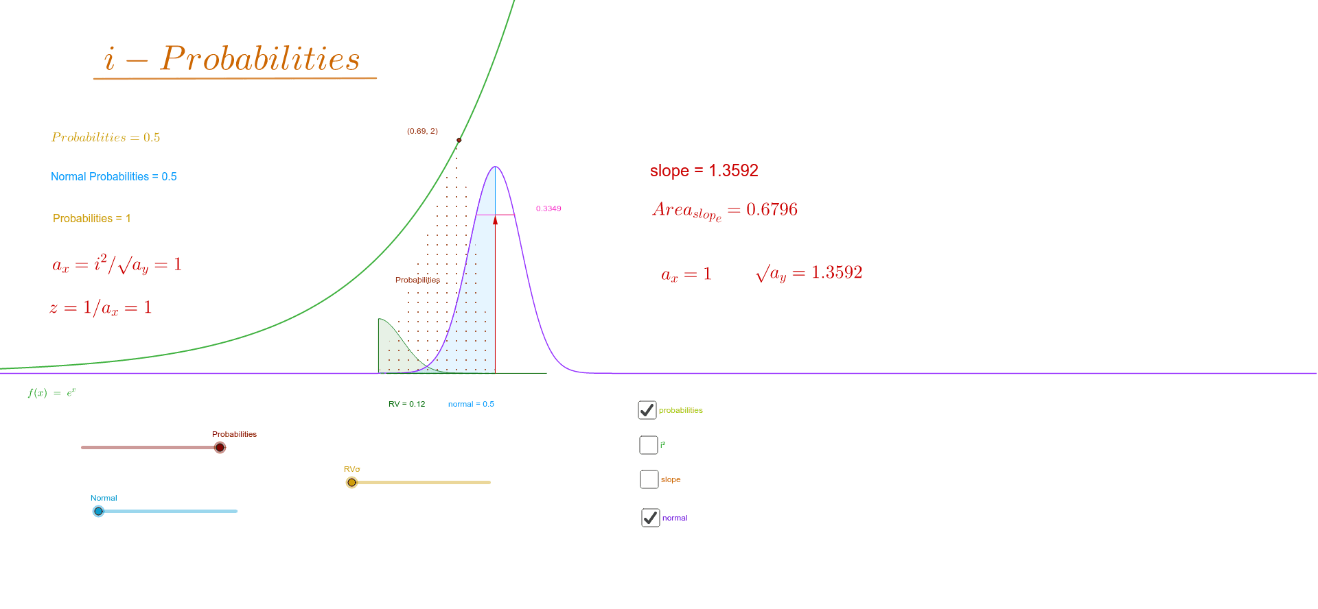
This example demonstrates how to use geometric shapes and probability distributions together to create reference points for understanding the normal distribution. Key mathematical concepts include probability and statistics, geometric construction, and graphing functions. Construction involves using GeoGebra commands such as Vector, Segment, Point, Polygon, Circle, Area, etc. Suitable for high school students or college students learning probability statistics and geometric construction.
GeoGebra Commands & Parameters
Vector((d, 0)) → uVector((d, 0), (d, c)) → vSegment(B, A) → tPoint(u) → CPolygon(B, A, C) → poly1, c_1, b_1, a_xPoint(v) → DPolygon(B, D, C) → poly2, c_2, b_2, d_1Vector((d, 0), (d, b)) → wPoint(w) → ECircle(B, C) → qCircle(B, E) → hCircle(B, D) → kArea(k) → rPointIn(k) → PointkArea(h) → jPointIn(h) → PointhArea(q) → lPointIn(q) → PointqIntegral(p, 0, 0.851) → RVIntegral(s, 0, 1) → normalSegment(F, G) → ePoint(w) → HOrthogonalLine(H, w) → iPoint(i) → IPoint(i) → JSegment(I, J) → a_1OrthogonalLine(E, w) → e_1Point(e_1) → KSegment(K, E) → f_1Mirror(K, g_1) → K'Mirror(E, g_1) → E'Segment(K', E') → h_1Point(f_1) → MPoint(h_1) → NSegment(M, N) → j_1Point(h_1) → LSegment(B, L) → k_1Slope(k_1) → slopePoint(l_1) → PPolygon(B, P, O) → poly3, o_1, b_3, p_1