
Practice: Second Order Derivatives
Loading the math board and drawing, please wait…
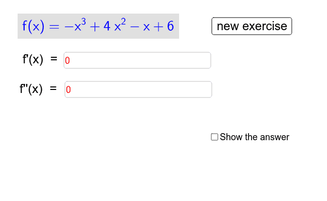
This example demonstrates the concept of second order derivatives. It involves core mathematical concepts such as derivatives and is constructed using GeoGebra commands like Shuffle, Random, Element, Simplify, and Derivative. Suitable for high school mathematics education and learning the application of second order derivatives.
GeoGebra Commands & Parameters
Shuffle({-1, 1}) → lijstaRandom(-8, 8) → dRandom(-8, 8) → cRandom(-8, 8) → bElement(lijsta, 1) → aSimplify((a * x^(3)) + (b * x^(2)) + (c * x) + d) → fDerivative(f) → ggDerivative(gg) → gIf(a < 0, "+", "-") → teklIf(a < 0, "-", "+") → tekrIf(a < 0, "convex", "concave") → teko3If(a < 0, "concave", "convex") → teko1Textfield(ant) → FirstTextfield(ante) → secondIf(ant ≟ gg ∧ ante ≟ g, "Correct!", "Try Again") → text3
AI Drawing Prompt Reference
Draw a function and its second derivative, showing the change in concavity. Generate a cubic function with random coefficients, then compute its first and second derivatives. Label the concavity intervals based on the sign of the second derivative and display the correct concavity description on the graph. Finally, show a message 'Correct!' if the first and second derivative graphs are accurate, otherwise 'Try Again'.
The prompt above was compiled from the original drawing commands and is for reference only.