
Position Vectors and Scalar Multiples of Vectors
Loading the math board and drawing, please wait…
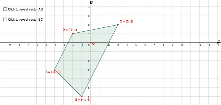
This example demonstrates the geometric representation of position vectors and their scalar multiples, showing how vector direction and magnitude change with scalar factors. Core mathematical concepts include vector definition, position vectors (from origin), scalar multiplication (stretching/shrinking), vector addition and polygon closure, and collinearity conditions. Construction highlights: using GeoGebra commands Polygon to build quadrilateral poly1, Vector to create vectors a, b, c, d, u, v, and Intersect to find intersection points; objects include points A, B, C, D, O, and multiple text labels (text1 to text12) for annotations. Suitable for high school or early college vector geometry lessons, helping students intuitively grasp the geometric meaning of vector operations and explore linear combinations and polygon properties.
GeoGebra Commands & Parameters
Polygon(A, B, C, D) → poly1, a, b, c, dVector(A, D) → uVector(B, C) → vIntersect(xAxis, yAxis) → OVector(O, A) → wVector(O, D) → eVector(O, B) → fVector(O, C) → g
AI Drawing Prompt Reference
Draw a quadrilateral ABCD and connect its diagonals AC and BD. Mark the origin O and draw vectors OA, OD, OB, and OC from O. Then, draw vector u from A to D and vector v from B to C. Finally, find the intersection of the x-axis and y-axis as the origin O and label vectors w, e, f, and g, representing vectors from O to A, D, B, and C respectively.
The prompt above was compiled from the original drawing commands and is for reference only.