
Population Logistic Slope Field - First Order Differential Equations
Loading the math board and drawing, please wait…
In collections
Differential equation Material
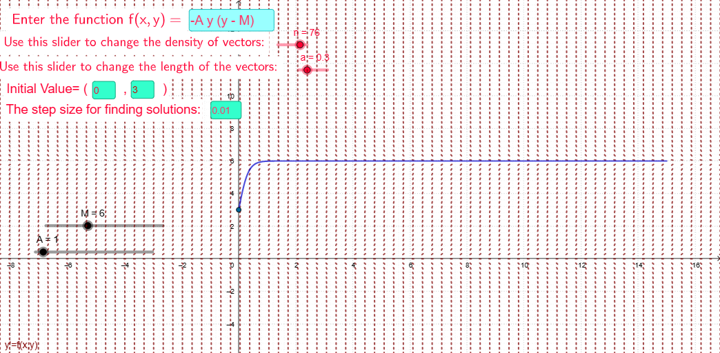
This example illustrates the application of first-order differential equations in a population logistic growth model. Key mathematical concepts include first-order differential equations and slope fields. Using commands like SlopeField and SolveODE in GeoGebra, the slope field and solutions to the differential equation are constructed. Suitable for high school mathematics education and students learning differential equations.
GeoGebra Commands & Parameters
Textfield(f) → InputBox1SlopeField(f, n, a) → slopefield1Textfield(a) → InputBox2Textfield(c) → InputBox3Textfield(d) → InputBox4Textfield(b) → InputBox5SolveODE(f, c, d, 15, b) → numericalIntegral1
AI Drawing Prompt Reference
Draw a graph of a population logistic growth slope field. The graph should include a slope field showing the slope changes of a differential equation. Key points like initial values and growth rates should be labeled. The construction order: first draw the slope field, then label key points, and finally show the solution curve.
The prompt above was compiled from the original drawing commands and is for reference only.