
Polynomial Functions Exploration
Loading the math board and drawing, please wait…
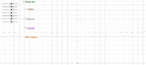
This example demonstrates the properties and graphs of polynomial functions. It involves core concepts of polynomial functions such as coefficients, roots, and derivatives. By adjusting the coefficients of the polynomial, you can observe changes in the graph. The example uses GeoGebra commands for polynomial functions, slider animations, and geometric constructions.
GeoGebra Commands & Parameters
Numeric a(1)Numeric b(1)Numeric c(1)Numeric d(1)Numeric e(1)Numeric f(1)Numeric g(1)h(x) = (a * x^(6)) + (b * x^(5)) + (c * x^(4)) + (d * x^(3)) + (e * x^(2)) + (f * x) + gp(x) = (a * x^(5)) + (b * x^(4)) + (c * x^(3)) + (d * x^(2)) + (e * x) + fq(x) = (a * x^(4)) + (b * x^(3)) + (c * x^(2)) + (d * x) + er(x) = (a * x^(3)) + (b * x^(2)) + (c * x) + ds(x) = (a * x^(2)) + (b * x) + cNumeric a_1(1)Numeric b_1(1)Numeric c_1(1)Numeric d_1(1)Numeric a_2(1)Numeric b_2(1)Boolean i(false)Boolean j(false)Boolean k(false)Boolean l(false)Boolean m(false)
AI Drawing Prompt Reference
Draw the graphs of a polynomial function and its first to fifth derivatives, with six adjustable coefficients controlled by sliders, showing how changes in coefficients affect the graphs, and the positions of the roots of the function and its derivatives, with geometric constructions to aid in understanding the properties of polynomial functions.
The prompt above was compiled from the original drawing commands and is for reference only.