
Polyhedra with Equivalent Vertices and Extreme Distribution on a Common Sphere
Loading the math board and drawing, please wait…
In collections
₈Polyhedra with extreme distribution of equivalent vertices
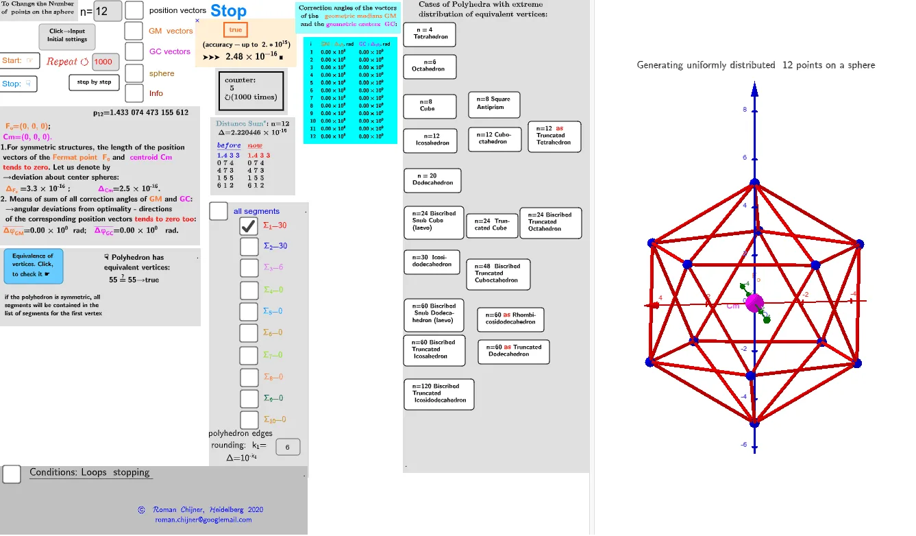
① This example demonstrates a special class of polyhedra whose vertices are all equivalent (symmetrically equivalent) and exhibit an extreme distribution on the same sphere, such as optimizing distances, centroid, or volume. ② Core mathematical concepts include polyhedral symmetry, spherical geometry, centroid/barycenter, optimization problems (linear programming or linear optimization), geometric mean, median value, volume, and special points like the circumsphere center. ③ Construction highlights: from the construction summary, GeoGebra commands such as Sphere, Text/Textfield, TableText, Append, Zip, If, and Sum are used, along with objects like O (center), R (radius), n (number of vertices), p1 (vertex list), Wii_P (weights), Cm (centroid), aPV/aGM/aGC (area, geometric mean, geometric center related quantities). Interactive input boxes (InputBox) allow parameter adjustment to dynamically observe how vertex distribution changes on the sphere. ④ Suitable for high school to university level solid geometry, optimization, and mathematical modeling, as well as visual exploration of symmetric polyhedra in computer graphics.
GeoGebra Commands & Parameters
LaTeX(Um1) → lll1_1LaTeX(Um0) → lll0Sphere(O, R) → p1Textfield(n) → InputBox1Textfield(i0) → InputBox2Text(r) → TxtrTextfield(k_1) → InputBox4UnicodeToLetter(34) → u34Textfield(k_2) → InputBox5TableText(ltxt0, ltxt1, "v") → textltxt01Append(A, Sequence[((random(), random(), random()) * R), i, 2, n]) → l2sText(("(up\; to\; 10^{-15})\;\\ accuracy= " * ScientificText[cc, 3]), C, true, true) → text5rZip(Vector[a, a + UnitVector[a]], a, lP') → lVector1Textfield(scale) → InputBox6TableText(Append["i", 1…n], Append[" \fgcolor{orange}{GM :Δφ_i}, rad", l1], Append["\fgcolor{magenta}{GC :Δφ_i} , rad", l1c], "v") → text23Text("\;\;\;\;\;\;\;\;\;\;\;\;\;\fgcolor{" + (If[c', "orange", "brown"]) + "} \boxed{ " + c' + "}\;\;\;\; \;\;\;\;\; \\\;\; ( accuracy- up\; to\;\; 2.*10^{" + k_2 + ("\;})\;\\\;\; ➤➤➤\;\;\;\scalebox{1.3}{ " + (ScientificText[cc, 3])) + "}\;█ ", C, true, true) → text9If(bu, "Animation", "Stop") → bue0Zip(Vector[a, a + (1.5 * UnitVector[b])], a, lP', b, Wi_P) → lVector3Zip(Vector[a, a + (1.5 * UnitVector[b])], a, lP', b, Wi_Pc) → lVector2TableText({Join[{{"n"}, Sequence[i, i, 4, 69 + 3]}], Join[{{" p_n=P_n/[R*n*(n-1)/2]"}, lp}]}, "vl") → txt_lpText("" + Um1) → txt_pSum(Flatten[Sequence[Append[Sequence[Element[txt_p, i], i, m1(k), m2(k)], " "], k, 1, 5]]) → txtUm1Zip(Segment[Element[lP', y(a)], Element[lP', z(a)]], a, ll1bb(1)) → ll1Zip(Segment[Element[lP', y(a)], Element[lP', z(a)]], a, ll1bb(2)) → ll2Zip(Segment[Element[lP', y(a)], Element[lP', z(a)]], a, ll1bb(3)) → ll3
AI Drawing Prompt Reference
Draw a sphere with a labeled center and radius. On the same common sphere, place a set of n vertices (points) that all lie on the sphere’s surface, with n and additional parameters such as i, k1, k2, and scale provided as adjustable inputs. Display annotation text showing an accuracy note, and include a table or text panel that reports per-vertex distribution quantities like GM :Δφ_i and GC :Δφ_i together with corresponding radial values. Finally, construct and show line segments derived from the distribution results to visually emphasize the extreme vertex distribution on the sphere, keeping the parameter controls active for observing how the configuration changes.
The prompt above was compiled from the original drawing commands and is for reference only.