
Polar Points of Intersection Demo
Loading the math board and drawing, please wait…
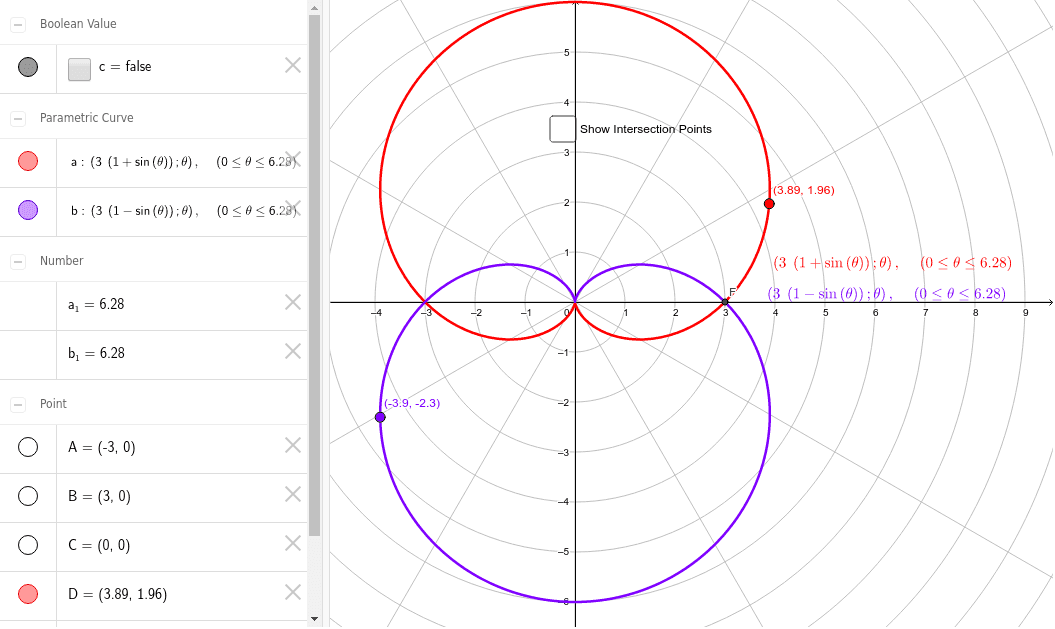
This example demonstrates the calculation and visualization of intersection points in polar coordinates. It involves core math concepts like polar coordinates, curve intersections, and analytical geometry. Key GeoGebra commands used are CurveCartesian for plotting curves, Intersect for finding intersections, and Point for labeling them, with objects a, b, A, B, C, D, E, F, c. Suitable for high school students and math enthusiasts learning polar coordinates and analytical geometry.
GeoGebra Commands & Parameters
CurveCartesian(((3 * (1 + sin(θ))); θ), θ, 0, (2 * 3.141592653589793)) → aCurveCartesian(((3 * (1 - sin(θ))); θ), θ, 0, (2 * 3.141592653589793)) → bIntersect(a, b, 3.151468067365083, 3.1517180381123944) → AIntersect(a, b, 3.387369593679059E-6, 3.387369593679059E-6) → BIntersect(a, b, 4.71238898038469, 1.570796326794897) → CPoint(a) → DPoint(b) → EIntersect(a, b, 0.163902597322425, 6.141755649419573) → F
AI Drawing Prompt Reference
Draw two polar curves: one is 3 times (1 plus sine of theta), the other is 3 times (1 minus sine of theta), both from 0 to 2π. Mark all intersection points, including the coincident point near the origin, the symmetric top and bottom points, and the side intersections. Also place one arbitrary point on each curve. Show the symmetric crossing pattern clearly with highlighted intersection markers.
The prompt above was compiled from the original drawing commands and is for reference only.