Polar Intersections: Dynamic Loci and Conditional Probability Interaction

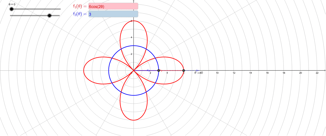
This example demonstrates the dynamic intersection points of two polar curves (functions f_1 and f_2 controlled by parameter θ), allowing real-time adjustment of parameters via sliders and input boxes to observe the generation of intersection loci. Core mathematical concepts include polar equations, curve intersections, loci, and the geometric representation of conditional probability, along with reflections, inequalities, and scalene triangle properties. Construction highlights: uses GeoGebra's Locus command to generate intersection trajectories, Textfield and InputBox for interactive input, Segment and Vector for auxiliary constructions, with objects such as θ, f_1, r_1, A, loc1, InputBox1, r, k, u, text1, f_2, r_2, B, loc2, InputBox2, s, K. Suitable for high school or early college students to understand the dynamic nature of polar curve intersections, and for math lab sessions exploring parameter effects on intersection positions, as well as interdisciplinary applications with probability and statistics.