
Polar Coordinate Function Exploration
Loading the math board and drawing, please wait…
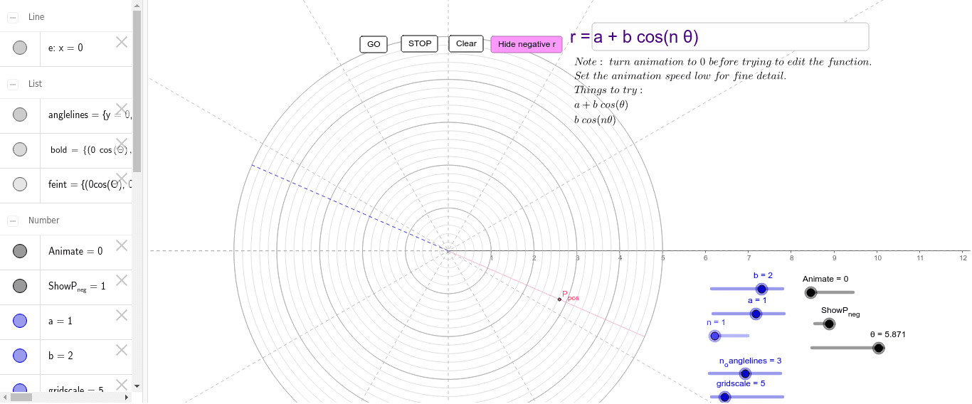
This example demonstrates how to draw and explore function graphs in polar coordinates. Key math concepts include the definition of polar coordinates, function graphing, and the application of parametric equations. Construction highlights involve commands like Sequence, Segment, Textfield, and objects such as n, θ, b, a, gridscale, anglelines, Animate, etc. It is suitable for high school and above students to understand the properties and variations of polar coordinate functions.
GeoGebra Commands & Parameters
Sequence(y = tan(Θ) * x, Θ, 0, 3.141592653589793, π / (2 * n_{o}anglelines)) → anglelinesSequence(CurveCartesian[r * cos(Θ), r * sin(Θ), Θ, 0, 6.28319], r, 0, gridscale, 1) → boldSequence(CurveCartesian[r * cos(Θ), r * sin(Θ), Θ, 0, 6.28319], r, 0, gridscale, 0.2) → feintSegment((0, 0), -Q) → dSegment((0, 0), Q) → cTextfield(r) → inputBox1
AI Drawing Prompt Reference
Draw polar coordinate function graphs, showing lines radiating from the origin and concentric circles of varying thickness, along with angle lines generated using the tangent function, and include a text box for inputting the radius value, presenting the characteristics of function graphs in polar coordinates.
The prompt above was compiled from the original drawing commands and is for reference only.