
Polar Conics with Eccentricity and Directrix
Loading the math board and drawing, please wait…
In collections
Conics Doug Kuhlmann
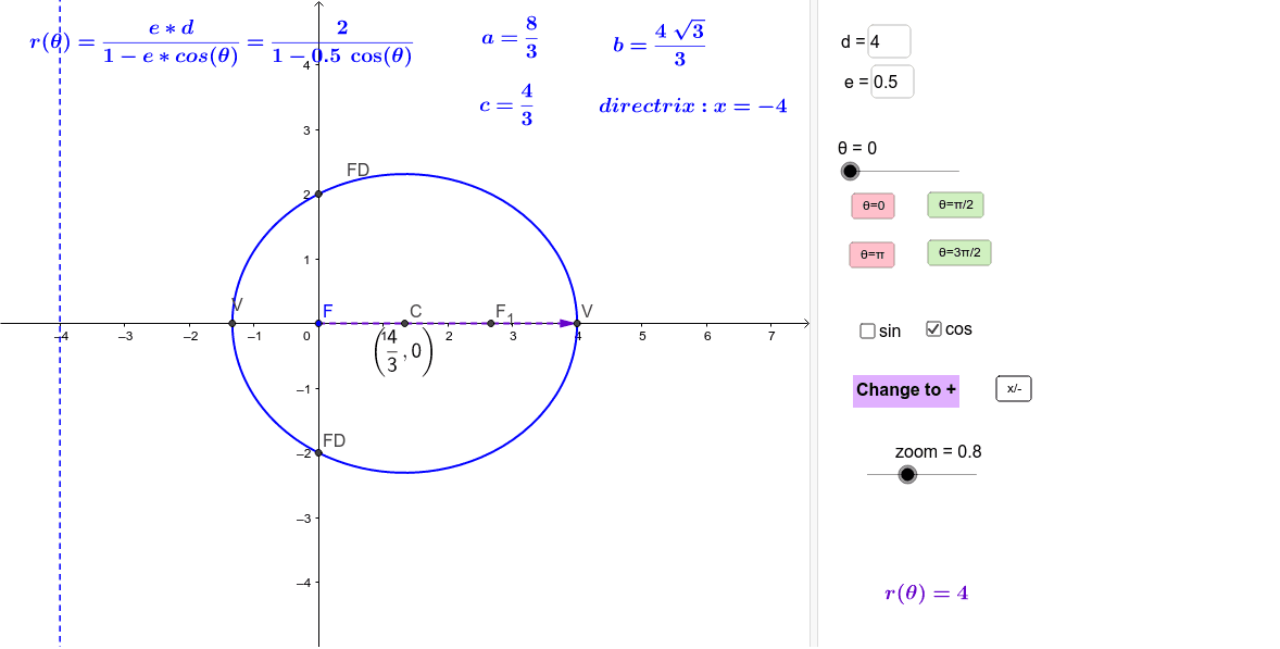
This example demonstrates conic sections (ellipse, hyperbola, parabola) in polar coordinates, visually illustrating the geometric significance of eccentricity and directrix. Key math concepts include polar equations, eccentricity, directrix, and properties of quadratic curves. GeoGebra commands used are CurveCartesian for plotting, Vector for vectors, If for conditional logic, Max/Min for extrema, Textfield for text display, and SurdText for radical formatting. Suitable for high school coordinate geometry education, helping students grasp the definitions and properties of conic sections and enhancing mathematical modeling skills.
GeoGebra Commands & Parameters
CurveCartesian((rc(t) * cos(t)), (rc(t) * sin(t)), t, 0, 6.283185307179586) → rcpVector(rcp(θ)) → uIf(togneg ≟ 0, "+", "-") → tgnIf(togneg ≟ 1, "Change to +", "Change to -") → PlusMinusCurveCartesian((rs(t) * cos(t)), (rs(t) * sin(t)), t, 0, 6.28319) → rspVector(rsp(θ)) → wMax({x(Vc_1), x(Vc_2), x(Vs_1), x(Vs_2)}) → MaxXMin({x(Vc_1), x(Vc_2), x(Vs_1), x(Vs_2)}) → MinXMax({y(Vc_1), y(Vc_2), y(Vs_1), y(Vs_2)}) → MaxYMin({y(Vc_1), y(Vc_2), y(Vs_1), y(Vs_2)}) → MinYIf(sn, x(Cs), x(Cc)) → xCenIf(sn, y(Cs), y(Cc)) → yCenMax(abs(MaxX), abs(MinX)) → MXMax(abs(MaxY), abs(MinY)) → MYTextfield(ecc) → eEQTextfield(dtrx) → dEQMin(abs(y(Vs_1)), abs(y(Vs_2))) → FVsMin(abs(x(Vc_1)), abs(x(Vc_2))) → FVcIf(SIGN < 0, Cs + (0, csi), Cs - (0, csi)) → FsIf(SIGN < 0, Cc + (csi, 0), Cc - (csi, 0)) → FcSurdText(Cc) → CcValueSurdText(Cs) → CsValue