
Piecewise Function Graphing
Loading the math board and drawing, please wait…
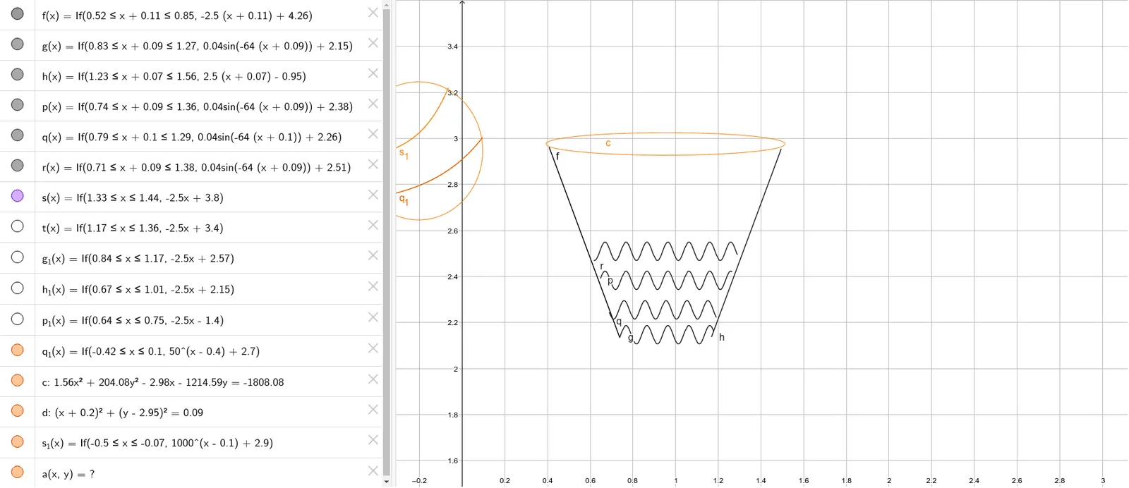
This example demonstrates the graph of a piecewise function. It involves concepts such as piecewise functions, integration, and quadratic equations. Using GeoGebra commands like f, g, h, etc., the graph of a piecewise function can be constructed. Suitable for high school mathematics education and learning.
GeoGebra Commands & Parameters
f(x) = If[0.52 ≤ x + 0.11210001289469079 ≤ 0.85, (-2.5 * (x + 0.11210001289469079)) + 4.260244322883237]g(x) = If[0.83 ≤ x + 0.09152538389309472 ≤ 1.27, (0.04 * sin((-64 * (x + 0.09152538389309472)))) + 2.1469426032522003]h(x) = If[1.2342 ≤ x + 0.06537527420935363 ≤ 1.5599, (2.5 * (x + 0.06537527420935363)) - 0.946563800038152]p(x) = If[0.74 ≤ x + 0.09152538389309495 ≤ 1.355, (0.04 * sin((-64 * (x + 0.09152538389309495)))) + 2.383259915422688]q(x) = If[0.79 ≤ x + 0.1002420871210089 ≤ 1.29, (0.04 * sin((-64 * (x + 0.1002420871210089)))) + 2.255013117067864]r(x) = If[0.71 ≤ x + 0.09152538389309484 ≤ 1.38, (0.04 * sin((-64 * (x + 0.09152538389309484)))) + 2.509400943054016]s(x) = If[1.3296 ≤ x ≤ 1.44, (-2.5 * x) + 3.8]t(x) = If[1.1718 ≤ x ≤ 1.36, (-2.5 * x) + 3.4]g_1(x) = If[0.8391 ≤ x ≤ 1.169, (-2.5 * x) + 2.57]h_1(x) = If[0.6674 ≤ x ≤ 1.0124, (-2.5 * x) + 2.15]p_1(x) = If[0.64 ≤ x ≤ 0.7504, (-2.5 * x) - 1.4]q_1(x) = If[-0.415 ≤ x ≤ 0.0952, 50^(x - 0.4) + 2.7](1.5625 * x^(2)) + (204.08163 * y^(2)) - (2.9776 * x) - (1214.58822 * y) = -1808.07866(x + 0.20436)^(2) + (y - 2.9457)^(2) = 0.09s_{1}(x) = If[-0.4981 ≤ x ≤ -0.0657, 1000^(x - 0.1) + 2.9]a(x, y) = NaN
AI Drawing Prompt Reference
Draw a piecewise function graph with multiple linear segments and one parabolic segment. The linear segments are: y = -2.5x + 4.26 (x from 0.74 to 1.355), y = -2.5x + 3.8 (x from 1.3296 to 1.44), y = -2.5x + 3.4 (x from 1.1718 to 1.36), y = -2.5x + 2.57 (x from 0.8391 to 1.169), y = -2.5x + 2.15 (x from 0.6674 to 1.0124), y = -2.5x - 1.4 (x from 0.64 to 0.7504), and y = 50^(x - 0.4) + 2.7 (x from -0.415 to 0.0952). The parabolic segment is defined by the equation 1.5625x^2 + 204.08163y^2 - 2.9776x - 1214.58822y + 1808.07866 = 0, with a center at (-0.20436, 2.9457) and a radius of 0.09.
The prompt above was compiled from the original drawing commands and is for reference only.