
Phase Portrait of Linear DEs with Real Distinct Eigenvalues #2
Loading the math board and drawing, please wait…
In collections
Differential Equations
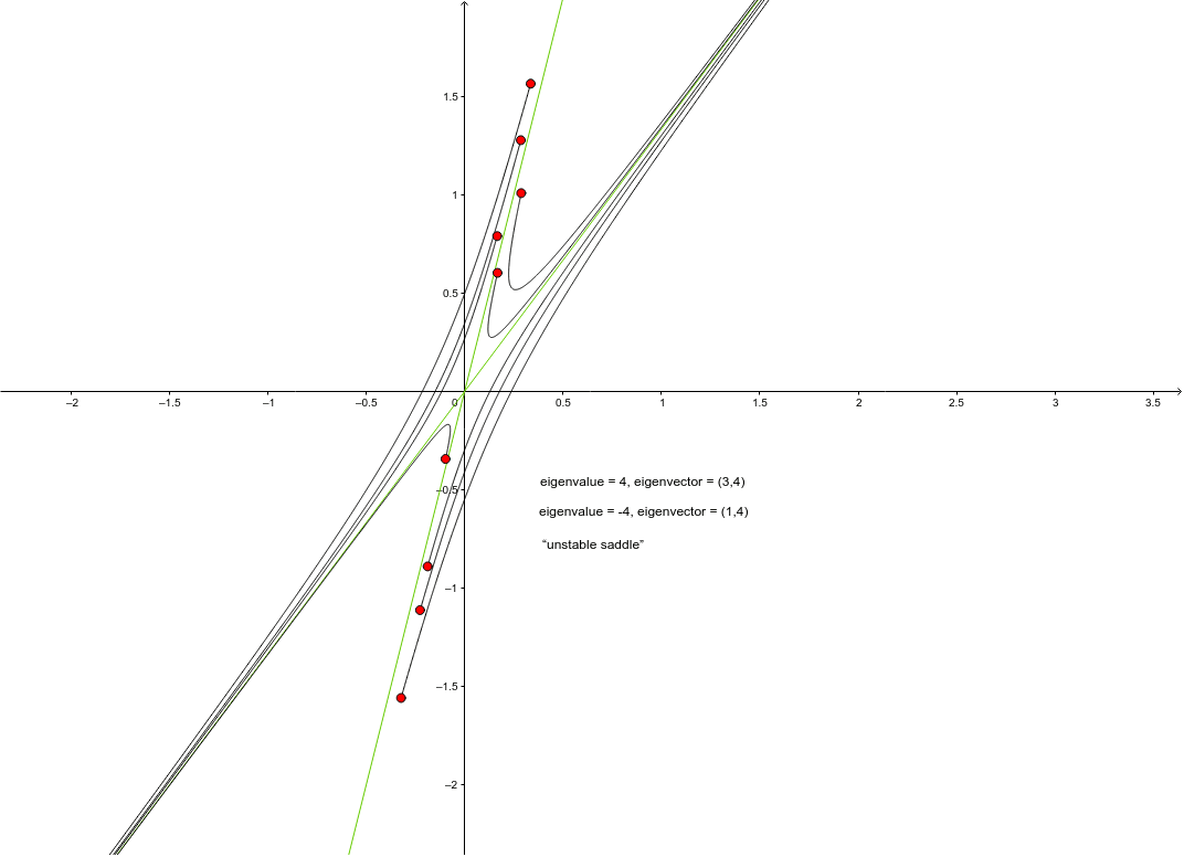
This example demonstrates the phase portrait of a linear system of differential equations with constant coefficients featuring two real, distinct eigenvalues leading to an unstable outcome. Key math concepts include linear differential equations, eigenvalues, phase portraits, and stability analysis. The construction utilizes GeoGebra commands like SolveODE, Intersect, and Line as outlined in the summary. Ideal for university-level mathematics courses or differential equations learning.
GeoGebra Commands & Parameters
SolveODE(g, f, x(A), y(A), 10, 0.001) → numericalIntegral1SolveODE(g, f, x(D), y(D), 10, 0.001) → numericalIntegral2SolveODE(g, f, x(E), y(E), 10, 0.001) → numericalIntegral3SolveODE(g, f, x(B), y(B), 10, 0.001) → numericalIntegral4SolveODE(g, f, x(C), y(C), 10, 0.001) → numericalIntegral5SolveODE(g, f, x(G), y(G), 10, 0.001) → numericalIntegral7SolveODE(g, f, x(H), y(H), 10, 0.001) → numericalIntegral6SolveODE(g, f, x(F), y(F), 10, 0.001) → numericalIntegral8SolveODE(g, f, x(I), y(I), 10, 0.001) → numericalIntegral9Intersect(xAxis, yAxis) → JLine(J, K) → aLine(J, L) → b