
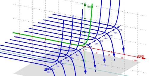
Phantom Graph of exp(x)
Loading the math board and drawing, please wait…
In collections
Phantom Graphs
This example demonstrates the phantom graph of the exponential function exp(x). It involves key mathematical concepts such as functions, derivatives, and image transformations. Using GeoGebra commands like Plane, Intersect, and Sequence, the positive and negative parts of the exponential function are constructed, allowing for the observation of its graph characteristics. Suitable for high school mathematics education and learning.
GeoGebra Commands & Parameters
Plane((0, c, 0), (1, c, 1), (-1, c, 3)) → aIntersect(f, l, (-1.2039728043259361, 0.3)) → ASequence((log(abs(c)), c, (n * π)), n, -7, 7, 2) → PtsNegSequence((log(c), c, (n * π)), n, 2, 6, 2) → PtsPosSequence((log(c), c, (n * π)), n, -6, -2, 2) → PtsPos2Sequence(CurveCartesian[u, ((-1)^(n) * ℯ^(u)), (n * π), u, -25, 25], n, -7, -1) → PGNegSequence(CurveCartesian[u, ((-1)^(n) * ℯ^(u)), (n * π), u, -25, 25], n, 1, 7) → PGsPos
AI Drawing Prompt Reference
Draw the graph of the exponential function exp(x), including its positive and negative parts. First, draw a plane, then find the intersection point A between the function and the plane. Next, use a series of sequence commands to generate key points on the negative and positive halves of the axis, and finally, use these points to draw the positive and negative parts of the exponential function's graph.
The prompt above was compiled from the original drawing commands and is for reference only.