
Phantom Graph for Ax^4+Bx^2+C
Loading the math board and drawing, please wait…
In collections
Phantom Graphs
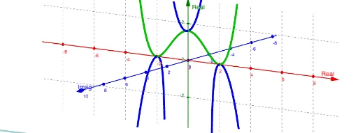
This example demonstrates the phantom graph of the quartic function Ax^4+Bx^2+C, highlighting its shape and key features. Core math concepts include function graphing, special points, difference and slope, definite integral, and unit circle. Construction involves GeoGebra commands like ComplexRoot, Plane, and CurveCartesian, utilizing objects such as c, f, g, z_1, etc. Ideal for high school and advanced learners exploring complex function transformations and properties.
GeoGebra Commands & Parameters
ComplexRoot(f(x) - c) → z_1, z_2, z_3, z_4Plane((0, c, 0), (1, c, 1), (-2, c, 3)) → aCurveCartesian(0, (0.1 * (t^(4) + (8 * t^(2)) + 16)), t, t, -50, 50) → bCurveCartesian(t, (1.6 * t^(2)) - (0.4 * t^(4)), sqrt(t^(2) - 4), t, -25, 25) → jCurveCartesian(t, (1.6 * t^(2)) - (0.4 * t^(4)), (-sqrt(t^(2) - 4)), t, -25, 25) → k
AI Drawing Prompt Reference
Draw the phantom graph of a quartic function, highlighting its shape and key features, including function graph, special points, difference and slope, definite integral, and unit circle. First, plot the function graph, then add dashed lines for special points, and finally display the definite integral and unit circle.
The prompt above was compiled from the original drawing commands and is for reference only.