
Pedal Surface of Sphere
Loading the math board and drawing, please wait…
In collections
surface 3D /3D-Oberflächen 1
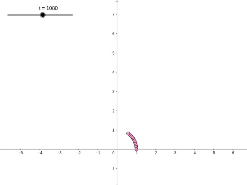
This example demonstrates the pedal surface of a sphere. It involves parametric equations and loci. Using GeoGebra commands such as OrthogonalLine, Intersect, and Sequence, the pedal surface of a sphere can be constructed. Suitable for high school mathematics education and learning.
GeoGebra Commands & Parameters
OrthogonalLine(B, a_1) → fIntersect(f, a_1) → CSequence(((cos(Mod[(a * 2), 180]° - 90°) * cos((Div[(a * 2), 180]° * 5))), (cos(Mod[(a * 2), 180]° - 90°) * sin((Div[(a * 2), 180]° * 5))), sin(Mod[(a * 2), 180]° - 90°)), a, 1, t) → 리스트1Sequence(Intersect[OrthogonalLine[B, (x(((cos(Mod[(a * 2), 180]° - 90°) * cos((Div[(a * 2), 180]° * 5))), (cos(Mod[(a * 2), 180]° - 90°) * sin((Div[(a * 2), 180]° * 5))), sin(Mod[(a * 2), 180]° - 90°))) * (x - x(((cos(Mod[(a * 2), 180]° - 90°) * cos((Div[(a * 2), 180]° * 5))), (cos(Mod[(a * 2), 180]° - 90°) * sin((Div[(a * 2), 180]° * 5))), sin(Mod[(a * 2), 180]° - 90°))))) + (y(((cos(Mod[(a * 2), 180]° - 90°) * cos((Div[(a * 2), 180]° * 5))), (cos(Mod[(a * 2), 180]° - 90°) * sin((Div[(a * 2), 180]° * 5))), sin(Mod[(a * 2), 180]° - 90°))) * (y - y(((cos(Mod[(a * 2), 180]° - 90°) * cos((Div[(a * 2), 180]° * 5))), (cos(Mod[(a * 2), 180]° - 90°) * sin((Div[(a * 2), 180]° * 5))), sin(Mod[(a * 2), 180]° - 90°))))) + (z(((cos(Mod[(a * 2), 180]° - 90°) * cos((Div[(a * 2), 180]° * 5))), (cos(Mod[(a * 2), 180]° - 90°) * sin((Div[(a * 2), 180]° * 5))), sin(Mod[(a * 2), 180]° - 90°))) * (z - z(((cos(Mod[(a * 2), 180]° - 90°) * cos((Div[(a * 2), 180]° * 5))), (cos(Mod[(a * 2), 180]° - 90°) * sin((Div[(a * 2), 180]° * 5))), sin(Mod[(a * 2), 180]° - 90°))))) = 0], (x(((cos(Mod[(a * 2), 180]° - 90°) * cos((Div[(a * 2), 180]° * 5))), (cos(Mod[(a * 2), 180]° - 90°) * sin((Div[(a * 2), 180]° * 5))), sin(Mod[(a * 2), 180]° - 90°))) * (x - x(((cos(Mod[(a * 2), 180]° - 90°) * cos((Div[(a * 2), 180]° * 5))), (cos(Mod[(a * 2), 180]° - 90°) * sin((Div[(a * 2), 180]° * 5))), sin(Mod[(a * 2), 180]° - 90°))))) + (y(((cos(Mod[(a * 2), 180]° - 90°) * cos((Div[(a * 2), 180]° * 5))), (cos(Mod[(a * 2), 180]° - 90°) * sin((Div[(a * 2), 180]° * 5))), sin(Mod[(a * 2), 180]° - 90°))) * (y - y(((cos(Mod[(a * 2), 180]° - 90°) * cos((Div[(a * 2), 180]° * 5))), (cos(Mod[(a * 2), 180]° - 90°) * sin((Div[(a * 2), 180]° * 5))), sin(Mod[(a * 2), 180]° - 90°))))) + (z(((cos(Mod[(a * 2), 180]° - 90°) * cos((Div[(a * 2), 180]° * 5))), (cos(Mod[(a * 2), 180]° - 90°) * sin((Div[(a * 2), 180]° * 5))), sin(Mod[(a * 2), 180]° - 90°))) * (z - z(((cos(Mod[(a * 2), 180]° - 90°) * cos((Div[(a * 2), 180]° * 5))), (cos(Mod[(a * 2), 180]° - 90°) * sin((Div[(a * 2), 180]° * 5))), sin(Mod[(a * 2), 180]° - 90°))))) = 0], a, 1, t) → 리스트2
AI Drawing Prompt Reference
Draw the pedal surface of a sphere. Start with a fixed point outside the sphere. Take a series of points on the sphere, distributed according to a parametric equation. For each point on the sphere, construct a plane passing through the fixed point and perpendicular to the line connecting that point to the sphere's center. Find the intersection of this plane with the sphere. As the parameter varies, these intersection points trace a spatial curve, and the collection of such curves forms the pedal surface. The figure should show the sphere, the fixed point, and the resulting surface, highlighting its parametric and locus nature.
The prompt above was compiled from the original drawing commands and is for reference only.