Curve of Intersection of Two Spheres

Loading the math board and drawing, please wait…

2016-08-29 18:01

In collections intersection: surface-surface, curve-curve intersection: surface-surface, curve-curve intersection: surface-surface, curve-curve intersection: surface-surface, curve-curve

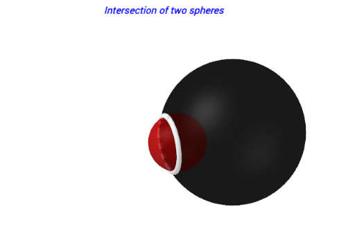
This GeoGebra example demonstrates the three-dimensional curve formed by the intersection of two spheres, visualized through parametric equations and the Sequence command. The core mathematical concepts include solid geometry (sphere equations), solving the intersection of two spheres (which yields a circle or spatial curve), and parametric representation of curves. Construction highlights: variables R, r, dx control sphere radii and center distance; LaTeX formulas define the parametric equations of the intersection curve; the Sequence command generates a point list (list1) along the curve; text objects display key parameters. Suitable for high school or early college students learning spatial curves, sphere intersections, and parametric equations, as well as for dynamic geometry demonstrations in mathematics labs.

GeoGebra Commands & Parameters

Sequence(CurveCartesian[x0, (i * fy_z(t)), t, t, (-max_t), max_t], i, -1, 1, 2) → list1
LaTeX(a, false, false) → text3
LaTeX(b, false, false) → text4

AI Drawing Prompt Reference

Draw two spheres that partially overlap, with adjustable radii and center distance. The intersection forms a spatial curve (a circle or more complex curve), which should be represented by parametric equations. Generate a sequence of points along this curve to highlight its path. Label the key parameters such as radii and center distance, and display their values as text. The scene should clearly show the spheres, the intersection curve, and the parameter points in 3D space, suitable for educational demonstration.

The prompt above was compiled from the original drawing commands and is for reference only.