
Partial Derivatives by Andrew Brown
Loading the math board and drawing, please wait…
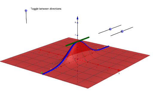
This example demonstrates the concept of partial derivatives. Partial derivatives are the rates of change of a multivariable function in a specific direction. Using commands like Segment, Point, and CurveCartesian in GeoGebra, the example constructs the function graph and calculates the partial derivatives. Suitable for university calculus courses.
GeoGebra Commands & Parameters
Segment((8, -3, 6), (8, 3, 6)) → bbbPoint(bbb) → BBBSegment((6, -3, 6), (6, 3, 6)) → aaaPoint(aaa) → AAACurveCartesian(t, b, (3 * ℯ^((-(t^(2) + (0.1 * b^(2)))))), t, -10, 10) → rCurveCartesian(t, b, (m * (t - a)) + c, t, a - 3, a + 3) → t_1CurveCartesian(t, d, (m * (t - a)) + c, t, a - 3, a + 3) → tSegment((-6, -5, 6), (-6, -5, 8)) → cccPoint({(-6, -5, 6), (-6, -5, 8)}) → CCCCurveCartesian(a, t, (3 * ℯ^((-(a^(2) + (0.1 * t^(2)))))), t, -10, 10) → pCurveCartesian(a, t, (n * (t - b)) + c, t, b - 3, b + 3) → q
AI Drawing Prompt Reference
Draw a 3D function graph with the equation 3 * ℯ^(-(x^2 + 0.1 * y^2)), where x and y range from -10 to 10. Then, draw the tangent lines at points (8,0,6) and (6,0,6), and at x=3 and y=3. Finally, draw the tangent lines at x=0 and y=0.
The prompt above was compiled from the original drawing commands and is for reference only.