Parametrizing the Intersection of a Cylinder and z=xy

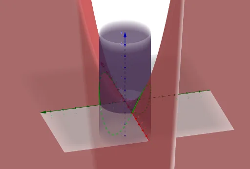
This example demonstrates how to parameterize and visualize the intersection curve between a cylinder and the surface z = xy in 3D. It highlights key ideas from solid analytic geometry: curve–surface intersection, using equation constraints to derive a parametric representation, and expressing the resulting intersection as a parametric Cartesian space curve. The construction proceeds by enforcing the cylinder’s implicit relation on (x, y), substituting into z = xy to obtain z, and then building the corresponding 3D curve in GeoGebra. The GeoGebra workflow is centered on the command “CurveCartesian,” along with the involved objects (f, a, b, c, eq1) that encode the parameterization and the defining equations. Suitable for high-school advanced geometry/analytic geometry, as well as early undergraduate calculus/analytic geometry learning and modeling exercises.