
Parametric Curves in Space by Brian Abbott
Loading the math board and drawing, please wait…
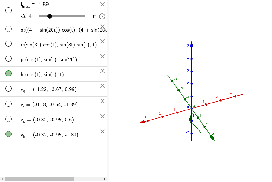
This example demonstrates the plotting and dynamic behavior of parametric curves in 3D space. Key math concepts include parametric equations, vector operations, and coordinate geometry. It is constructed using GeoGebra commands like CurveCartesian for curve plotting and Vector for vector creation, with objects such as t_{tmax}, q, r, p, h, and velocity vectors v_{q}, v_{r}, v_{p}, v_{h} for parameter control and dynamic visualization. Ideal for university calculus courses or spatial geometry learning.
GeoGebra Commands & Parameters
CurveCartesian((((4 + sin((20 * t))) * cos(t)), ((4 + sin((20 * t))) * sin(t)), cos((20 * t))), t, (-π), t_{tmax}) → qCurveCartesian((sin((3 * t)) * cos(t)), (sin((3 * t)) * sin(t)), t, t, (-π), t_{tmax}) → rCurveCartesian((cos(t), sin(t), sin((2 * t))), t, (-π), t_{tmax}) → pCurveCartesian((cos(t), sin(t), t), t, (-π), t_{tmax}) → hVector(q(t_{tmax})) → v_{q}Vector(r(t_{tmax})) → v_{r}Vector(p(t_{tmax})) → v_{p}Vector(h(t_{tmax})) → v_{h}
AI Drawing Prompt Reference
In 3D space, draw four parametric curves starting from negative pi to a variable terminal parameter. The first curve is a torus-like spiral with a sinusoidal radius variation, creating a flower-like ring. The second is a 3D rose curve with three petals in the horizontal plane and a linear rise in the vertical direction. The third is a circular wave with a vertical sine oscillation. The fourth is a standard helix rising uniformly. At the end of each curve, draw a vector from the origin to that endpoint, representing the position vector. All curves and vectors together illustrate the dynamic behavior of parametric equations in space.
The prompt above was compiled from the original drawing commands and is for reference only.