Original Data of Way 1 & Way 2: Visualizing Non-Constant Variance

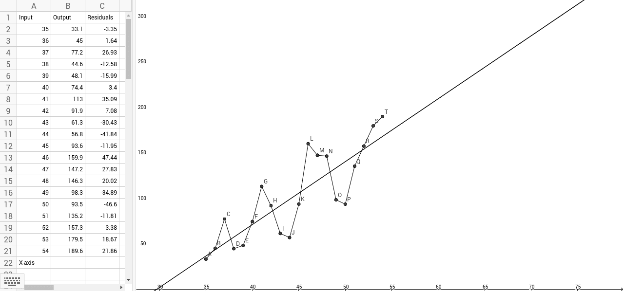
This GeoGebra dataset is designed to visualize and analyze the non-constant variance of errors (heteroscedasticity) within regression models. The core mathematical concepts demonstrated include variance, residuals, linear fitting, and the geometric representation of error terms. To construct the visualizations, the dataset defines coordinate points from A1 to A14, B1 to B14, and C1 to C14. The GeoGebra command FitLineY is used to compute the regression lines, while the Segment command constructs line segments that highlight the changing width of the error intervals. This example is ideal for high school or college students and educators studying statistics, econometrics, and linear regression, providing a practical tool to understand the diagnostics of OLS assumptions.