Orbit Lab 3.1: Elliptical Planetary Motion and Kepler's Laws

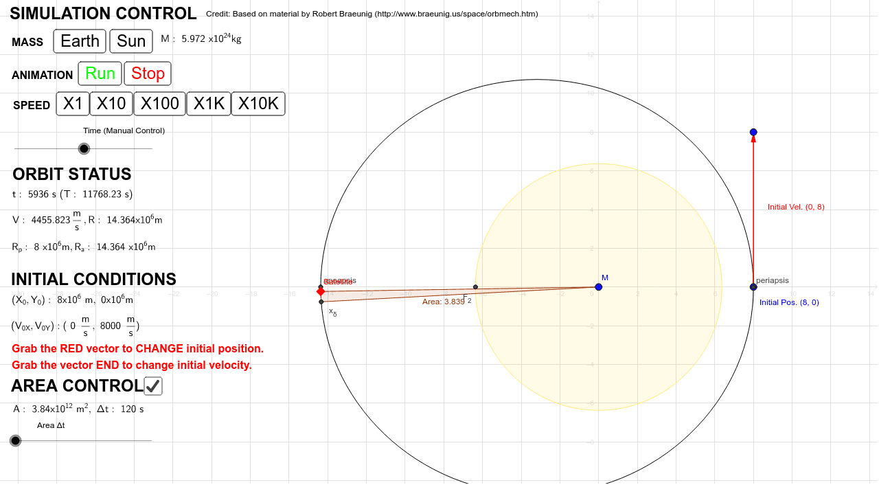
① This example demonstrates the elliptical orbit of a planet (Earth) around the Sun (a focus), with dynamic visualization of orbital parameters, velocity vectors, and area sweeping in real time. ② Core mathematical concepts include ellipse geometry (foci, semi-major/minor axes, eccentricity), Kepler's second law (constant areal velocity), vector operations, velocity and acceleration decomposition in differential geometry, and numerical simulation with time stepping and interpolation. ③ Construction highlights: from the summary, the GeoGebra commands used include Vector, Min, Max, Ellipse, If, Mod, Intersect, Ray, Polygon, and Circle, with objects such as M_sun, M_earth, F_1/F_2 (foci), e (eccentricity), T (period), v_0 (initial velocity), and a slider δ_t controlling the time step to update position and velocity dynamically. ④ Suitable for high school physics (universal gravitation and celestial motion) and introductory university astronomy, as well as mathematics classes teaching parametric equations and polar coordinates of ellipses, providing an intuitive understanding of orbital mechanics and geometric properties.