
Opaque Cone
Loading the math board and drawing, please wait…
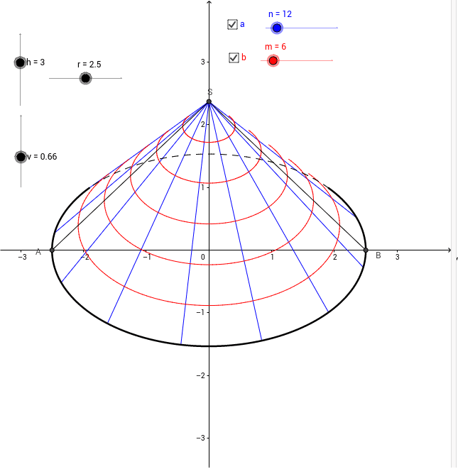
This example demonstrates a 3D model of an opaque cone, involving core math concepts like solid geometry, coordinate geometry, parametric equations, and function graphing. It utilizes GeoGebra commands such as CurveCartesian, Point, Conic, Tangent, Intersect, Segment, Sequence, Defined, ClosestPoint, and PathParameter for construction, suitable for high school and above learning 3D shapes and geometric modeling.
GeoGebra Commands & Parameters
CurveCartesian((r * cos(t)), ((r * sin(t)) * sin(v)), t, 0, 6.283185307179586) → ePoint(e) → EPoint(e) → DPoint(e) → CConic(B, C, D, E, A) → fTangent(S, f) → g, iIntersect(f, i) → FSegment(A, S) → b_1Segment(B, S) → a_1Sequence(CurveCartesian[((r * (1 - i / h)) * cos(t)), (((r * (1 - i / h)) * sin(t)) * sin(v)) + (i * cos(v)), t, 0, 6.283185307179586], i, 0, h, h / m) → liste3Defined(F) → jSequence(Segment[S, ((r * cos(i)), ((r * sin(i)) * sin(v)))], i, 0, 6.283185307179586, (2 * π / n)) → liste1ClosestPoint(e, F) → FFPathParameter(FF) → pfIntersect(f, g) → GClosestPoint(e, G) → GGPathParameter(GG) → pgSequence(Segment[S, Point[e, i - floor(i)]], i, pg, 1 + pf, 1 / n) → liste2CurveCartesian((r * cos(t)), ((r * sin(t)) * sin(v)), t, ang, anf) → eeCurveCartesian((r * cos(t)), ((r * sin(t)) * sin(v)), t, anf - (2 * π), ang) → eeeSequence(CurveCartesian[((r * (1 - i / h)) * cos(t)), (((r * (1 - i / h)) * sin(t)) * sin(v)) + (i * cos(v)), t, ang, anf], i, 0, h, h / m) → liste6Sequence(CurveCartesian[(((kxx * r) * (1 - i / h)) * cos(t)) + (((kyx * r) * (1 - i / h)) * sin(t)), (((kxy * r) * (1 - i / h)) * cos(t)) + (((kyy * r) * (1 - i / h)) * sin(t)) + (kzy * i), t, ang, anf], i, 0, h, h / m) → liste7
AI Drawing Prompt Reference
Draw a 3D model of an opaque cone, highlighting its geometric structure. Begin by sketching the cone's lateral surface using parametric equations, showing the tapering edges from base to apex. Then, add the base and apex of the cone, along with several generatrix lines connecting them. Finally, use curves to link the lateral surface to the base, creating a complete cone with a clear three-dimensional appearance and geometric construction.
The prompt above was compiled from the original drawing commands and is for reference only.