
One Variable Linear Equations Practice
Loading the math board and drawing, please wait…
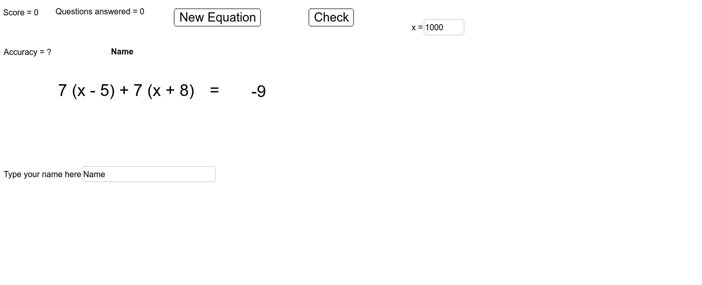
This example demonstrates the solution process of one-variable linear equations. Key mathematical concepts include the methods of solving one-variable linear equations. Using GeoGebra commands such as RandomElement, Random, FractionText, Textfield, etc., it dynamically generates problems and shows the solution steps. Suitable for middle school math education.
GeoGebra Commands & Parameters
RandomElement({1, 1, 1, 1, 2, 3, 4}) → a_4Random(-10, 10) → a_3RandomElement({-10, -9, -8, -7, -6, -5, -4, -3, -2, -1, 1, 2, 3, 4, 5, 6, 7, 8, 9, 10}) → a_1Random(-10, 10) → a_2Random(-10, 10) → b_1Random(-10, 10) → b_3Random(-10, 10) → c_1Random(-10, 10) → c_4Random(-10, 10) → d_2Random(-10, 10) → d_4Random(-10, 10) → d_5RandomElement({1, 3}) → a_{1n}RandomElement({2, 4}) → a_{1d}RandomElement({-10, -9, -8, -7, -6, -5, -4, -3, -2, -1, 1, 2, 3, 4, 5, 6, 7, 8, 9, 10}) → c_3RandomElement({-10, -9, -8, -7, -6, -5, -4, -3, -2, -1, 1, 2, 3, 4, 5, 6, 7, 8, 9, 10}) → c_2RandomElement({-10, -9, -8, -7, -6, -5, -4, -3, -2, -1, 0, 1, 2, 3, 4, 5, 6, 7, 8, 9, 10, 0.5, 0.25, 0.75}) → d_3RandomElement({-10, -9, -8, -7, -6, -5, -4, -3, -2, -1, 1, 2, 3, 4, 5, 6, 7, 8, 9, 10}) → d_1FractionText(a_{1n} / a_{1d}) → fraca1RandomElement({-10, -9, -8, -7, -6, -5, -4, -3, -2, 2, 3, 4, 5, 6, 7, 8, 9, 10}) → b_2RandomElement({-10, -9, -8, -7, -6, -5, -4, -3, -2, -1, 1, 2, 3, 4, 5, 6, 7, 8, 9, 10}) → a_{r1}Random(-10, 10) → a_{r2}Random(1, 13) → problemnumberTextfield(check) → InputBox1Text((a_1 * x) + a_2) → Problem1LText(a_3) → Problem1RText(a_3) → Problem2RText(x + a_2) → Problem2LText(a_2 + (a_1 * x)) → Problem3LText(a_3) → Problem3RText((a_1 * ((a_4 * x) + a_2))) → Problem4LText(a_3) → Problem4RText(x + b_1) → Problem5LAText(b_2) → Problem5LBText(b_3) → Problem5RText(c_1 + (c_2 * (x + c_3))) → Problem6LText(c_4) → Problem6RText((d_1 * (x + d_2)) + (d_3 * (x + d_4))) → Problem7LText(d_5) → Problem7RText((a_1 * x) + a_2) → Problem8LText((a_{r1} * x) + a_{r2}) → Problem8RText((a_1 * x) + a_2) → Problem9LText(a_{r2} + (a_{r1} * x)) → Problem9RText(a_2 + (a_1 * x)) → Problem10LText(a_{r2} + (a_{r1} * x)) → Problem10RText((a_1 * (x + a_2))) → Problem11LText((a_{r1} * (x + a_{r2}))) → Problem11RText(c_1 + (c_2 * (x + c_3))) → Problem12LText((a_{r1} * x) + a_{r2}) → Problem12RText((d_1 * (x + d_2)) + (d_3 * (x + d_4))) → Problem13LText(c_1 + (c_2 * (x + c_3))) → Problem13RPoint(Circle[A, 170]) → BSegment(A, B) → aText(("Questions answered = " * numberofquestions)) → numberofquestionskeepText(("Accuracy = " * accuracy)) → accuracykeepText(("Score = " * score)) → scorekeepTextfield(name) → inputBox1
AI Drawing Prompt Reference
Create a dynamic one-variable linear equation practice interface displaying 12 different types of equations, each containing the unknown x. These equations include: standard form ax+b=c, fractional forms, polynomial forms with parentheses like a(bx+c)=d, distributive property forms like a(x+b)+c(x+d)=e, and equations with x on both sides like ax+b=cx+d. There is an input field at the top for students to check their answers. All coefficients and constants in the equations are randomly generated integers from -10 to 10, with simple fractions like 1/3 or 1/4. The layout is tidy with equations arranged in numbered order, clearly showing various typical forms of linear equations in one variable.
The prompt above was compiled from the original drawing commands and is for reference only.