
Normal Probability Plot
Loading the math board and drawing, please wait…
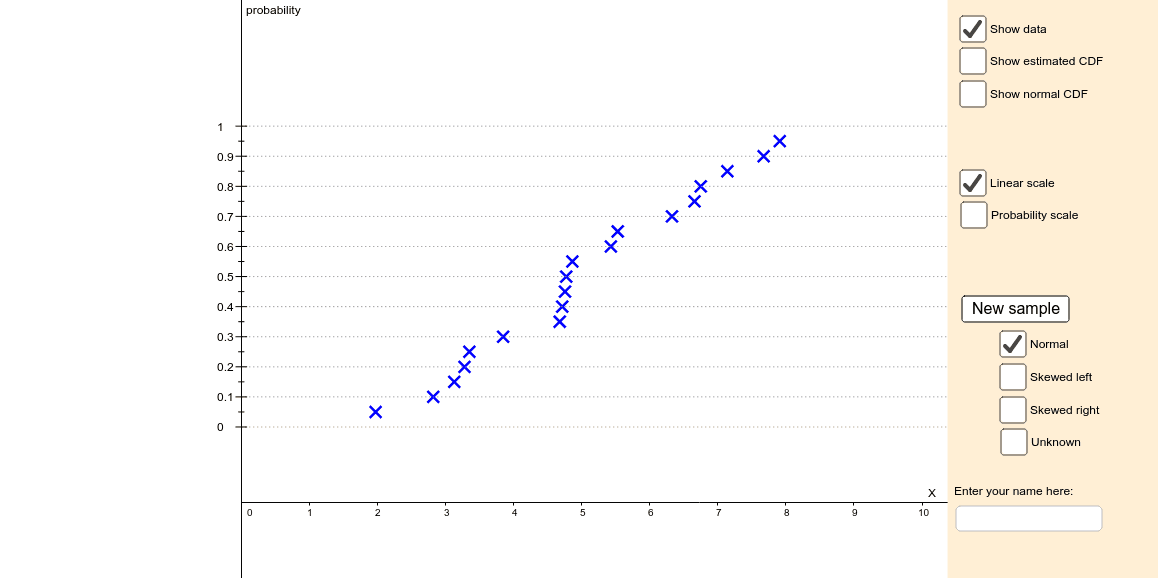
This applet demonstrates the relationship between a cumulative distribution function (CDF) plot and a probability plot. It smoothly animates the vertical quantile scale of a CDF plot into a probability plot. Key mathematical concepts include normal distribution in probability and statistics. Construction highlights the use of GeoGebra commands such as Sequence, Normal, Sort, Translate, etc. Suitable for teaching and learning probability and statistics.
GeoGebra Commands & Parameters
Sequence(RandomUniform[0, 10], i, 1, 19) → dataunifSequence(10 - InverseChiSquared[3, RandomUniform[0, 1]], i, 1, 19) → dataleftSequence(RandomNormal[5, 2], i, 1, 19) → datanormSequence(InverseChiSquared[3, RandomUniform[0, 1]], i, 1, 19) → datarightNormal(0.5, 1 / ((2 * InverseNormal[0, 1, scalept])), x) → normfSort(If[skewleft, dataleft, If[skewright, dataright, If[norm, datanorm, dataunif]]]) → dataTranslate(Rotate[Sequence[(xx, (2 * normf(xx))), xx, -3, 3, 0.05], 1.5708], (axescross - normoffset, 0)) → normpdfpointsMean(data) → xbarSampleSD(data) → sIf(probscale, t2, 1 - t2) → tSequence((0.05 * i), i, 0, 20) → ycoords1Zip(If[yy ≟ 0, -3, If[yy ≟ 1, 3, InverseNormal[0, 1, yy] / ((2 * InverseNormal[0, 1, scalept])) + 0.5]], yy, ycoords1) → ycoords2Zip(((1 - t) * aa) + (t * bb), aa, ycoords1, bb, ycoords2) → ycoordsSequence((Element[data, i], Element[ycoords, i + 2]), i, 1, 9) → altPointsJoin(Sequence[{(Element[data, i], Element[ycoords, i + 1]), (Element[data, i + 1], Element[ycoords, i + 1])}, i, 1, 19]) → ogivePointsPolyLine(ogivePoints) → ogiveZip(((1 - t) * yy) + (t * (InverseNormal[0, 1, yy] / ((2 * InverseNormal[0, 1, scalept])) + 0.5)), yy, Sequence[(0.1 * i) + 0.05, i, 0, 9]) → altycoordsPolygon({Corner[2], Corner[3], (x(Corner[3]) - (x(Corner[3]) - x(Corner[4])) / 5.5, y(Corner[3])), (x(Corner[2]) - (x(Corner[2]) - x(Corner[1])) / 5.5, y(Corner[2]))}) → fillerLine(normlineP1, normlineP2) → normdraglinePolygon(Join[{KeepIf[y(P) < y(normlineP1), P, normpdfpoints], {(axescross - (2 * normf(y(normlineP1))) - normoffset, y(normlineP1)), (axescross - normoffset, y(normlineP1))}}]) → normareaPolyLine(normpdfpoints) → normpdfSegment((0, -0.27), (0, -0.23)) → zerotickSequence((Element[data, i], Element[ycoords, i + 1]), i, 1, 19) → dataPointsSequence(Ray[(axescross, Element[ycoords, i]), (1, Element[ycoords, i])], i, 1, 21, 2) → gridlinesSequence(Text[zz, (axescross - normoffset + 0.06, zz / ((2 * InverseNormal[0, 1, scalept])) + 0.49)], zz, -3, 3) → zlabelsSegment((axescross - normoffset, y(normlineP1)), (axescross, y(normlineP1))) → normsegmentSequence(Segment[(axescross - normoffset - 0.04, zz / ((2 * InverseNormal[0, 1, scalept])) + 0.5), (axescross - normoffset + 0.04, zz / ((2 * InverseNormal[0, 1, scalept])) + 0.5)], zz, -3, 3) → zticksSequence(Segment[(axescross - 0.08, Element[ycoords, i]), (axescross + 0.08, Element[ycoords, i])], i, 1, 21, 2) → tickmarksSequence(Text[Element[ycoords1, i], (axescross - 0.36, Element[ycoords, i] - 0.015)], i, 1, 21, 2) → ticklabelsZip(Segment[(axescross - 0.04, yy), (axescross + 0.04, yy)], yy, altycoords) → alttickmarksTextfield() → inputBox1
AI Drawing Prompt Reference
Draw a probability plot that illustrates the relationship between a cumulative distribution function (CDF) and a probability plot. The plot includes data points generated from uniform, inverse chi-squared, and standard normal distributions, arranged in order. A CDF curve is drawn, along with points that map the data to a probability plot. A standard normal probability density curve is added as reference. The figure also includes zero point markers, grid lines, and labels to annotate data points and curves. The overall graphic should clearly show the correspondence between the CDF curve and the probability plot points, suitable for teaching probability and statistics.
The prompt above was compiled from the original drawing commands and is for reference only.