
Net of a Cone by Daryl Cox
Loading the math board and drawing, please wait…
In collections
Surface Area Discovery
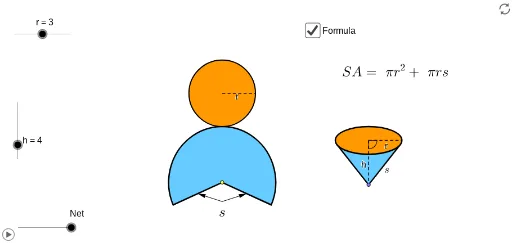
This example demonstrates the net of a cone and its surface area formula. It involves core mathematical concepts such as solid geometry, properties of cones, net development, and surface area calculation. The construction utilizes GeoGebra commands and objects like Point, Circle, Intersect, Ellipse, Vector, Translate, Arc, Segment, Angle, Line, Midpoint, If, Conic, OrthogonalLine, Tangent, Rotate, Center, Mirror, Polygon, CircleSector. It is suitable for high school students learning about the geometric properties and surface area formula of cones.
GeoGebra Commands & Parameters
Point(xAxis) → ACircle(A, r) → cIntersect(c, xAxis) → B, CEllipse(E, D, C) → eIntersect(xAxis, yAxis) → FVector(F, G) → uTranslate(B, Vector[(u * h)]) → B'_1Translate(C, Vector[(u * h)]) → C'_1Translate(A, Vector[(u * h)]) → A'_1Translate(e, Vector[(u * h)]) → e'_1Arc(e'_1, C'_1, B'_1) → p_5Arc(e'_1, B'_1, C'_1) → qSegment(A'_1, A) → h_6Segment(A'_1, C'_1) → pAngle(A, A'_1, C'_1) → αLine(A, A'_1) → jIntersect(e'_1, j) → H, ICircle(I, r) → tIntersect(t, j, 2) → KCircle(K, I) → d_1Intersect(d_1, j, 2) → NVector(H, N) → vTranslate(H, Vector[(v * n)]) → H'_1Translate(D, Vector[(u * h)]) → D'Translate(E, Vector[(u * h)]) → E'Line(B, B'_1) → lLine(C, C'_1) → mIntersect(d_1, l, 1) → PIntersect(d_1, m, 1) → QVector(B'_1, P) → zVector(C'_1, Q) → u_1Translate(B'_1, Vector[(z * n)]) → B''Translate(C'_1, Vector[(u_1 * n)]) → C''Midpoint(B'_1, A'_1) → RMidpoint(B, A) → SLine(R, S) → a_1Intersect(q, a_1) → T,Intersect(d_1, a_1, 1) → UVector(T, U) → v_1Translate(T, Vector[(v_1 * n)]) → T'If(n ≟ 0.01, B'_1, If[n < 1, B'', P]) → B_1If(n ≟ 0.01, T, If[n < 1, T', U]) → D_1If(n ≟ 0.01, H, If[n < 1, H'_1, N]) → E_1If(n ≟ 0.01, C'_1, If[n < 1, C'', Q]) → F_1Conic(B_1, D_1, E_1, F_1, I) → g_1Conic(I, B_1, D_1, E_1, F_1) → h_1OrthogonalLine(I, j) → l_1OrthogonalLine(H, j) → b_2Intersect(m, l_1) → H_2Midpoint(H_2, C'_1) → I_2OrthogonalLine(C'_1, m) → i_2Segment(K, F_1) → m_4Translate(e, Vector[(u * h)]) → e'Tangent(A, e'_1) → a, bIntersect(e', b) → J, G_2Intersect(e', a) → L, R_2Segment(A, J) → fSegment(A, L) → gCircle(I, sqrt(h^(2) + r^(2))) → kIntersect(k, j, 1) → MCircle(M, sqrt(h^(2) + r^(2))) → sSegment(M, I) → iRotate(I, γ, M) → I'_1Rotate(I, (-γ), M) → I'_2OrthogonalLine(I'_2, i_2) → b_1Intersect(b_2, b_1) → OMidpoint(H, O) → VCircle(V, O) → c_1Vector(O, I'_2) → wCenter(g_1) → WSegment(W, F_1) → e_1Vector(H, A) → w_1Translate(H, Vector[(w_1 * (n - 1))]) → H'If(n < 1, H, If[n < 2, H', A]) → ZSegment(H, Z) → f_1Rotate(I, (-δ), M) → I'Vector(L, I') → z_1Translate(c_1, Vector[(w * (n - 2))]) → k_1Center(k_1) → A_1Intersect(k_1, j) → C_1, Q_1Rotate(C_1, (180° * (n - 2)), A_1) → G_1If(n < 2, H, If[n ≤ 3, G_1, I'_2]) → H_1Mirror(H_1, j) → I_1Translate(L, Vector[(z_1 * (n - 2))]) → L'If(n < 2, L, If[n ≤ 3, L', I']) → J_1Mirror(J_1, j) → K_1Conic(I_1, H_1, J_1, I, K_1) → p_1Vector(A, M) → i_1Translate(A, Vector[(i_1 * (n - 2))]) → A'If(n < 2, A, If[n ≤ 3, A', M]) → L_1Tangent(L_1, p_1) → j_1, m_1Intersect(p_1, m_1, 1) → M_1Intersect(p_1, j_1, 1) → N_1Polygon(L_1, M_1, N_1) → poly1, n_1, l_2, m_2Arc(p_1, N_1, M_1) → q_1Line(L_1, b_2) → r_1Intersect(p_1, r_1, 1) → O_1Intersect(p_1, r_1, 2) → P_1Arc(p_1, P_1, O_1) → s_1Polygon(L_1, O_1, I_1) → poly2, i_3, l_3, o_1Polygon(L_1, H_1, P_1) → poly3, p_2, l_4, h_2Arc(p_1, O_1, I_1) → t_1Arc(p_1, H_1, P_1) → c_2Segment(L_1, I_1) → a_2Segment(L_1, H_1) → d_2Arc(p_1, H_1, I_1) → e_2Polygon(I_1, L_1, H_1) → poly4, h_3, i_4, l_5CircleSector(M, I'_2, I'_1) → f_2CircleSector(M, I'_2, I'_1) → g_2Arc(p_1, H_1, I_1) → k_2Segment(M_1, L_1) → j_2Segment(N_1, L_1) → n_2Polygon(I_1, L_1, H_1) → poly5, h_4, i_5, l_6Arc(p_1, H_1, I_1) → q_2Polygon(J, A, L) → poly6, l_7, j_3, a_3Point(xAxis) → R_1OrthogonalLine(R_1, xAxis) → r_2Intersect(i_2, r_2) → S_1Circle(R_1, r) → s_2Intersect(s_2, xAxis) → T_1, U_1OrthogonalLine(T_1, i_2) → t_2OrthogonalLine(V_1, i_2) → b_3OrthogonalLine(W_1, i_2) → c_3Intersect(i_2, t_2) → Z_1Intersect(i_2, b_3) → A_2Intersect(i_2, c_3) → B_2Ellipse(A_2, B_2, Z_1) → d_3Tangent(R_1, d_3) → e_3, f_3Intersect(d_3, f_3, 1) → C_2Intersect(d_3, e_3, 1) → D_2Polygon(C_2, D_2, R_1) → poly7, r_3, c_4, d_4Ellipse(A_2, B_2, Z_1) → g_3OrthogonalLine(U_1, xAxis) → k_3Intersect(g_3, k_3) → E_2, J_2Segment(S_1, E_2) → m_3Segment(S_1, R_1) → n_3Intersect(d_3, m_3, 1) → F_2Midpoint(g) → K_2Midpoint(f_1) → L_2Point(j) → M_2Midpoint(I_1, A') → N_2Midpoint(A', H_1) → O_2Vector(M_2, N_2) → u_2Vector(M_2, O_2) → v_2Line(M_2, r_1) → p_3Point(p_3) → P_2Vector(P_2, K_2) → z_2Vector(P_2, L_2) → u_3Center(g_3) → Q_2Angle(F_2, Q_2, R_1) → εSegment(I_1, H_1) → q_3Intersect(k_2, q_3, 2) → S_2Point(poly7) → T_2
AI Drawing Prompt Reference
Draw the net of a cone, including the base circle, the arc of the ellipse representing the side surface, the vertex, the center of the base circle, the radius line of the base circle, the height of the cone, and the lines connecting the boundary of the net and the vertex. Start by drawing a circle, then draw its diameter, followed by the height of the cone, and finally draw the arc of the ellipse representing the side surface, and connect the lines of the net boundary and the vertex.
The prompt above was compiled from the original drawing commands and is for reference only.