
Multiple Models for Proper Fractions by hoganl
Loading the math board and drawing, please wait…
In collections
fifth grade fractions
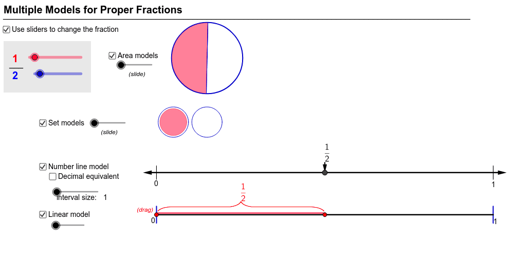
This example demonstrates how to display and compare proper fractions using various models including linear, number line, set, and area representations. Key math concepts involve fraction representation, number line, set theory, and area models. Construction highlights the use of GeoGebra commands like Segment, Point, Circle, Sequence, Max, Min, If, Polygon, Vector, Rotate, CircleSector along with objects such as num, denom, etc. Suitable for elementary and higher mathematics education to visually understand different representations of proper fractions.
GeoGebra Commands & Parameters
Segment(K_2, K_2 + (1 - num / denom, 0)) → linearModel1SegShiftPoint(linearModel1SegShift) → LinearModel1PtLCircle(R_1, T_1) → Circle_{model}Point(Circle[R_1, 0.105]) → C_2Sequence(If[round(flex * x(Element[list1, i]) / y(Element[list1, i])) / flex ≟ round(flex * x(L_1)) / flex, i, 0], i, 1, Length[list1]) → list2Max(list2) → matchMin(9 / denom, 1) → a9Min(4 / denom, 1) → a4Min(5 / denom, 1) → a5Min(8 / denom, 1) → a8Min(7 / denom, 1) → a7Min(6 / denom, 1) → a6Min(1 / denom, 1) → a1Min(2 / denom, 1) → a2If(denom < 10, " " + denom, "" + denom) → formatdMin(3 / denom, 1) → a3Min(10 / denom, 1) → a10Point(Circle[M, 1]) → QPoint(Circle[N, 1]) → RPoint(Circle[L_1, 0.02]) → U_1Point(Circle[U_1, 0.5]) → V_1Polygon(LinearModel1PtL + (0, -0.03), LinearModel1PtL + (num / denom, -0.03), LinearModel1PtL + (num / denom, 0.03), LinearModel1PtL + (0, 0.03)) → int1, a, b, c, eIf(impr > 1, 1, 0) → Rect_{show}Vector(NL_c, NL_l) → uVector(NL_c, NL_r) → vVector(FP_t, FP) → wIf(num / denom > 1, 1, 0) → Set_{show}Segment((1, 0.13), (1, 0.17)) → i_2Segment((0, 0.13), (0, 0.17)) → j_2Segment(R_1, C_2) → m_2Rotate(C_2, angle, R_1) → D_2CircleSector(R_1, C_2, D_2) → r_3Segment(R_1, D_2) → l_2Rotate(C_2, (360 / denom)°, R_1) → B_2Sequence(Segment[Rotate[C_2, (360 * i / denom)°, R_1], R_1], i, 0, denom) → Angle_{divseq}Segment(K_2, L_2) → a_2Vector((0, 0.25), (0.1, 0.25)) → image_{vector}Sequence(Translate[pic1, Vector[i * image_{vector}]], i, 0, denom - 1) → Set_{opencat}Sequence(Translate[pic2, Vector[i * image_{vector}]], i, 0, num - 1) → Set_{closedcat}Sequence(Translate[pic3, Vector[i * image_{vector}]], i, 0, denom - 1) → Set_{openstar}Sequence(Translate[pic4, Vector[i * image_{vector}]], i, 0, num - 1) → Set_{closedstar}Sequence(Segment[(0.045 + i / 11, 0.385), Point[Circle[(0.045 + i / 11, 0.59), 0]]], i, 0, denom) → Area_{rectdiv}Polygon(R_8, F_2, G_2, E_2) → rect_{red}, r_8, f_4, g_4, e_4Segment(R_8, I_2) → b_2Segment(E_2, H_2) → n_2Sequence(Segment[(0.045 + i / (3 * denom), 0.385), Point[Circle[(0.045 + i / (3 * denom), 0.59), 0]]], i, 0, denom) → Area_{rect2}Segment(E_2, M_2) → a_3Segment(J_2, R_8) → b_3Polygon(E_2, O_2, N_2, R_8) → poly1, e_5, o_2, n_3, r_4Segment(LinearModel1PtL + (0, 0.0050), LinearModel1PtR + (0, 0.0050)) → linearModel1LineSequence(Segment[(i, 0.13), (i, 0.17)], i, 0, 1, 1 / lineHashMarks) → lineHashMarkListSequence(Segment[(i, 0), (i, 0.05)], i, 0, 1, 1 / lineHashMarks) → linearHashMarkListSequence(Circle[(0.05 + i, 0.3), 0.045], i, 0, (denom - 1) / 10, 0.1) → setCircleOpenSequence(Circle[(0.05 + i, 0.3), 0.04], i, 0, (num - 1) / 10, 0.1) → setCircleShading