
Multiple Models for Proper Fractions by EDC Interactive Math
Loading the math board and drawing, please wait…
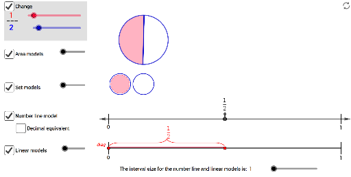
This example demonstrates proper fractions through various models including linear, number line, set, and area representations. Key math concepts involve fraction notation, number line interpretation, set theory, and area calculations. It is constructed using GeoGebra commands like Segment, Point, Circle, Polygon, Vector, Rotate, CircleSector, Sequence, and FractionText. Suitable for elementary and middle school mathematics education to visually understand different representations of proper fractions.
GeoGebra Commands & Parameters
Segment(K_2, K_2 + (1 - num / denom, 0)) → linearModel1SegShiftPoint(linearModel1SegShift) → LinearModel1PtLCircle(R_1, T_1) → Circle_{model}Point(Circle[R_1, 0.105]) → C_2Polygon(LinearModel1PtL + (0, -0.03), LinearModel1PtL + (num / denom, -0.03), LinearModel1PtL + (num / denom, 0.03), LinearModel1PtL + (0, 0.03)) → int1, a, b, c, eVector(NL_c, NL_l) → uVector(NL_c, NL_r) → vVector(FP_t, FP) → wSegment((1, 0.13), (1, 0.17)) → i_2Segment((0, 0.13), (0, 0.17)) → j_2Segment(R_1, C_2) → m_2Rotate(C_2, angle, R_1) → D_2CircleSector(R_1, C_2, D_2) → r_3Segment(R_1, D_2) → l_2Rotate(C_2, (360 / denom)°, R_1) → B_2Sequence(Segment[Rotate[C_2, ((360 * i / denom))°, R_1], R_1], i, 0, denom) → Angle_{divseq}Segment(K_2, L_2) → a_2Vector((0, 0.25), (0.1, 0.25)) → image_{vector}Sequence(Translate[pic1, Vector[(i * image_{vector})]], i, 0, denom - 1) → Set_{opencat}Sequence(Translate[pic2, Vector[(i * image_{vector})]], i, 0, num - 1) → Set_{closedcat}Sequence(Translate[pic3, Vector[(i * image_{vector})]], i, 0, denom - 1) → Set_{openstar}Sequence(Translate[pic4, Vector[(i * image_{vector})]], i, 0, num - 1) → Set_{closedstar}Polygon(R_8, F_2, G_2, E_2) → rect_{red}, r_8, f_4, g_4, e_4Segment(R_8, I_2) → b_2Segment(E_2, H_2) → n_2Segment(E_2, M_2) → a_3Segment(J_2, R_8) → b_3Polygon((0.045, 0.588), (0.045 + num / ((3 * denom)), 0.588), (0.045 + num / ((3 * denom)), 0.385), (0.045, 0.385)) → areaModel3polyFill, j, k, l, mPolygon((-0.4493678126189438, 0.486), (-0.0923678126189438, 0.486), (-0.0923678126189438, 0.656), (-0.4493678126189438, 0.656)) → fracBackground, d, f, g, hSegment(LinearModel1PtL + (0, 0.005), LinearModel1PtR + (0, 0.005)) → linearModel1LineSequence(Segment[(i, 0.13), (i, 0.17)], i, 0, 1, 1 / intervalHashMarks) → numLineHashMarksSequence(Segment[(i, 0), (i, 0.05)], i, 0, 1, 1 / intervalHashMarks) → linearHashMarksSequence(Circle[(0.05 + i, 0.3), 0.045], i, 0, (denom - 1) / 10, 0.1) → setCircleOpenSequence(Circle[(0.05 + i, 0.3), 0.04], i, 0, (num - 1) / 10, 0.1) → setCircleShadingSequence(Segment[(0.045 + i / 11, 0.388), (0.045 + i / 11, 0.588)], i, 0, denom) → Area_{rectdiv}Sequence(Segment[(0.044 + i / ((3 * denom)), 0.387), (0.044 + i / ((3 * denom)), 0.588)], i, 0, denom) → Area_{rect2}FractionText(1 / intervalHashMarks) → intervalValue
AI Drawing Prompt Reference
Draw a diagram showing proper fractions with linear, number line, set, and area models. Start by drawing a line segment to represent the numerator, and mark intervals on it for the number line. Then, use a circle and sectors to illustrate the area model, dividing the circle into equal parts based on the denominator and highlighting the numerator portion with different colors. Finally, represent the proper fraction with sets, using hollow circles for the excluded parts and solid circles for the included parts, arranged below the number line.
The prompt above was compiled from the original drawing commands and is for reference only.