
Multiple Geometric Views of a Single Fraction
Loading the math board and drawing, please wait…
In collections
The Fractions book
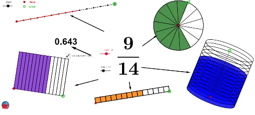
This example demonstrates how a single fraction can be visualized from several geometric perspectives. It covers core concepts such as geometric representation of fractions, proportional reasoning, coordinate geometry with segments and circles, and the use of sequences and vectors. The construction employs GeoGebra commands Circle, Point, Segment, Intersect, OrthogonalLine, Ellipse, Sequence, CurveCartesian, Line, Polygon, Element, CircleSector, Take, and Vector to build circular sectors, partitioned segments, vector translations, and dynamic sequences that enable switching between views. It is suitable for middle‑school fraction lessons, high‑school analytic geometry and vector introductions, and as a teaching resource for geometric construction and animation in GeoGebra.
GeoGebra Commands & Parameters
Circle(D, Zoom) → d_1Circle(D, (0.25 * Zoom)) → tCircle(D, (2 * Zoom)) → pPoint(p) → MSegment(D, M) → lIntersect(t, l) → Q,OrthogonalLine(D, l) → nIntersect(d_1, n) → N, OEllipse(N, O, Q) → bCircle(C, (2 * Zoom)) → qCircle(J, (3 * Zoom)) → kCircle(B, (4 * Zoom)) → fCircle(A, Zoom) → ePoint(e) → EPoint(f) → FSequence(Rotate[E, i, A], i, 0, 6.283185307179586, (2 * π / Den)) → liste1Sequence(Translate[B, Vector[(i * Vector[B, F])]], i, 0, 1, 1 / Den) → liste2Point(k) → KCurveCartesian(x(D) + (Zoom * cos(i)), y(D) + ((0.25 * Zoom) * sin(i)), i, 0, 6.28319) → b_1Sequence(Translate[J, Vector[(i * Vector[J, K])]], i, 0, 1, 1 / Den) → liste3Segment(B, F) → cCircle(A, E) → dSequence(Translate[b, Vector[(i * Vector[D, M])]], i, 0, 1, 1 / Den) → liste5Point(q) → GSegment(J, K) → jSequence(Polygon[Element[liste3, i], Element[liste3, i + 1], 4], i, 1, Length[liste3]) → liste3bSegment(C, G) → gOrthogonalLine(C, g) → hCircle(C, (1.5 * Zoom)) → sIntersect(s, h) → H, LLine(L, g) → iLine(G, h) → mIntersect(i, m) → IPolygon(C, G, I, L) → poly1, c_1, g_1, i_1, l_1Sequence(Translate[C, Vector[(i * Vector[C, G])]], i, 0, 1, 1 / Den) → liste4Sequence(Translate[L, Vector[(i * Vector[C, G])]], i, 0, 1, 1 / Den) → liste6Sequence(Segment[A, Element[liste1, i]], i, 1, Length[liste1]) → liste7Sequence(Segment[Element[liste4, i], Element[liste6, i]], i, 1, Length[liste6]) → liste8Element(liste1, Num + 1) → AACircleSector(A, E, AA) → e_1Element(liste2, Num + 1) → BBSegment(B, BB) → a_1Take(liste5, 1, Num + 1) → liste9Element(liste4, Num + 1) → CCElement(liste6, Num + 1) → LLPolygon(C, CC, LL, L) → poly2, c_2, cc, ll, l_2Take(liste3b, 1, Num) → liste10Line(M, n) → f_1Intersect(b, n) → P, RLine(R, l) → h_1Line(P, h_1) → j_1Intersect(f_1, h_1) → SIntersect(f_1, j_1) → TSegment(S, R) → k_1Segment(T, P) → m_1Vector(V, W) → uVector(Z, A_1) → vVector(B_1, C_1) → wVector(D_1, E_1) → zVector(F_1, G_1) → rCircle(D, pp) → p_1Intersect(p_1, l) → J_1,Sequence(Translate[b, Vector[(i * Vector[D, J_1])]], i, 0, 1, 0.01) → liste11Vector(K_1, L_1) → u_1
AI Drawing Prompt Reference
Visualize a fraction through multiple geometric perspectives. Start by drawing three concentric circles and an outer circle, then create a line segment and mark two intersection points. Construct an ellipse from these points and add several circles. Use rotation and vector translation to generate dynamic sequences, showing different geometric representations of the fraction. Finally, combine these elements through segmentation, connection, and dynamic transformations to illustrate the coordinate geometry and vector relationships of the fraction.
The prompt above was compiled from the original drawing commands and is for reference only.