
Move Points!
Loading the math board and drawing, please wait…
This example demonstrates how to explore spatial relationships by moving points. Key mathematical concepts include geometric transformations and functions. Using GeoGebra commands such as PointIn, Polygon, and FitPoly, students can intuitively understand the concepts of geometric transformations and functions. Suitable for middle school and above students for geometric construction and exploration.
GeoGebra Commands & Parameters
PointIn(i) → APointIn(b) → IPointIn(a) → EPolygon((x(E), y(E)), (x(A), y(A)), (x(I), y(I)), (x(E), y(I))) → Polígon1, p, q, r, f_1PointIn(a) → BPointIn(a) → CPointIn(a) → DPointIn(b) → FPointIn(b) → GPointIn(b) → HFitPoly({(y(A), z(A)), (y(F), z(F)), (y(G), z(G)), (y(H), z(H)), (y(I), z(I))}, 4) → fFitPoly({(x(A), z(A)), (x(B), z(B)), (x(C), z(C)), (x(D), z(D)), (x(E), z(E))}, 4) → gCurveCartesian(x(A), t, f(t), t, y(A), y(I)) → cCurveCartesian(t, y(A), g(t), t, x(E), x(A)) → dSurface(u, v, g(u) + f(v), u, x(E), x(A), v, y(A), y(I)) → eOrthogonalLine(E, xOyPlane) → jOrthogonalLine(I, xOyPlane) → kIntersect(j, xOyPlane) → JIntersect(k, xOyPlane) → KSurface(t + x(M) - x(L), s + y(M) - y(L), g(t) + f(s), t, x(E), x(A), s, y(A), y(I)) → lSurface((2 * x(A)) - u, v, g(u) + f(v), u, x(E), x(A), v, y(A), y(I)) → e_xSurface(u, (2 * y(A)) - v, g(u) + f(v), u, x(E), x(A), v, y(A), y(I)) → e_ySequence(Sequence[Surface[u + ((2 * k) * s), v + ((2 * l) * t), g(u) + f(v), u, x(E), x(A), v, y(A), y(I)], k, -2, 2], l, -2, 2) → l1Sequence(Sequence[Surface[(2 * x(A)) - u + ((2 * k) * s), v + ((2 * l) * t), g(u) + f(v), u, x(E), x(A), v, y(A), y(I)], k, -2, 2], l, -2, 2) → l2Sequence(Sequence[Surface[u + ((2 * l) * s), (2 * y(A)) - v + ((2 * k) * t), g(u) + f(v), u, x(E), x(A), v, y(A), y(I)], k, -2, 2], l, -2, 2) → l3Surface((2 * x(A)) - u, (2 * y(A)) - v, g(u) + f(v), u, x(E), x(A), v, y(A), y(I)) → e_{xy}Sequence(Sequence[Surface[(2 * x(A)) - u + ((2 * l) * s), (2 * y(A)) - v + ((2 * k) * t), g(u) + f(v), u, x(E), x(A), v, y(A), y(I)], k, -2, 2], l, -2, 2) → l4PointIn(Polígon1) → PPSequence(Sequence[((2 * x(A)) - x(PP) + ((2 * k) * s), y(PP) + ((2 * l) * t), g(x(PP)) + f(y(PP))), k, -2, 2], l, -2, 2) → lp2Sequence(Sequence[(x(PP) + ((2 * l) * s), (2 * y(A)) - y(PP) + ((2 * k) * t), g(x(PP)) + f(y(PP))), k, -2, 2], l, -2, 2) → lp3Sequence(Sequence[((2 * x(A)) - x(PP) + ((2 * l) * s), (2 * y(A)) - y(PP) + ((2 * k) * t), g(x(PP)) + f(y(PP))), k, -2, 2], l, -2, 2) → lp4Sequence(Sequence[(x(PP) + ((2 * k) * s), y(PP) + ((2 * l) * t), g(x(PP)) + f(y(PP))), k, -2, 2], l, -2, 2) → lp1
AI Drawing Prompt Reference
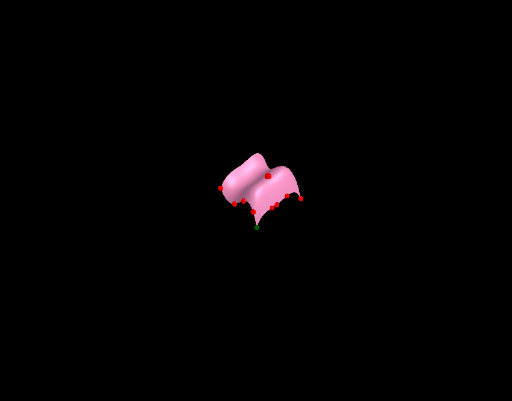
Draw a polygon using points A, B, C, D, E, F, G, H, and I, then fit polynomial functions f and g through these points. Next, draw curves c and d starting from points E and I respectively. Finally, draw surface e using points E and I, and create a series of surfaces l1 to l4 around these points.
The prompt above was compiled from the original drawing commands and is for reference only.