
Monte Carlo Pi Confidence Interval
Loading the math board and drawing, please wait…
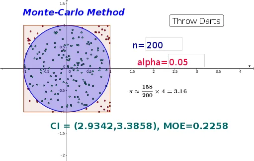
This example demonstrates how to estimate the value of Pi using the Monte Carlo method and shows the accuracy of the estimate through a confidence interval. Key math concepts include probability & statistics, definite integral, geometric probability, and confidence intervals. It uses GeoGebra commands like Sequence, Sum, Polygon, Zip, InverseNormal, and Textfield. Suitable for high school and above students to understand the application of probability statistics and calculus in geometric problems.
GeoGebra Commands & Parameters
Sequence(((2 * random()) - 1, (2 * random()) - 1), k, 1, n) → dartsSum(Zip[f(A), A, darts]) → successPolygon(A, B, C, D) → border, a, b, c, dZip(f(A), A, darts) → junkSequence(If[Element[junk, k], Element[darts, k]], k, 1, n) → list1InverseNormal(phat, sd, (0.5 * alpha)) → cilowInverseNormal(phat, sd, 1 - (0.5 * alpha)) → cihighTextfield(n) → inputBox1Textfield(alpha) → inputBox2
AI Drawing Prompt Reference
Estimate Pi using the Monte Carlo method by plotting random points within a square and a inscribed circle, showing the ratio of points inside the circle to estimate Pi and displaying a confidence interval. Generate random points, count those inside the circle, draw the square and circle, label the count of points inside the circle and total points, then show the confidence interval bounds.
The prompt above was compiled from the original drawing commands and is for reference only.