
Matching Histograms to Boxplots
Loading the math board and drawing, please wait…
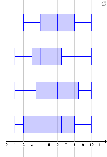
This example demonstrates how to visualize and compare data distributions using histograms and boxplots. Core math concepts include data distribution, median, quartiles, and probability & statistics. Constructed using GeoGebra commands like Frequency, Sequence, and BoxPlot. Suitable for high school mathematics teaching to help students understand data visualization techniques.
GeoGebra Commands & Parameters
Frequency(Sequence[11] - 0.5, A1:A40) → list1Sequence(Polygon[A + (i - 1, 0), A + (i, 0), A + (i, (k * list1(i))), A + (i - 1, (k * list1(i)))], i, 1, 10) → list1HFrequency(Sequence[11] - 0.5, B1:B40) → list2Frequency(Sequence[11] - 0.5, C1:C40) → list3Frequency(Sequence[11] - 0.5, D1:D40) → list4Sequence(Polygon[B + (i - 1, 0), B + (i, 0), B + (i, (k * list2(i))), B + (i - 1, (k * list2(i)))], i, 1, 10) → list2HSequence(Polygon[C + (i - 1, 0), C + (i, 0), C + (i, (k * list3(i))), C + (i - 1, (k * list3(i)))], i, 1, 10) → list3HSequence(Polygon[D + (i - 1, 0), D + (i, 0), D + (i, (k * list4(i))), D + (i - 1, (k * list4(i)))], i, 1, 10) → list4HSequence(Text[i, A + (i - 0.8, -0.8)], i, 1, 10) → text1Sequence(Text[i, B + (i - 0.8, -0.8)], i, 1, 10) → text2Sequence(Text[i, C + (i - 0.8, -0.8)], i, 1, 10) → text3Sequence(Text[i, D + (i - 0.8, -0.8)], i, 1, 10) → text4BoxPlot(2, 1, A1:A40) → aBoxPlot(6, 1, B1:B40) → bBoxPlot(10, 1, C1:C40) → cBoxPlot(14, 1, D1:D40) → d