Mapping Diagrams: Functions with Complex Parameters - Circles

Loading the math board and drawing, please wait…

2017-05-29 08:47

Circle Function Complex Number

In collections Mapping Diagrams to Visualize Complex Analysis

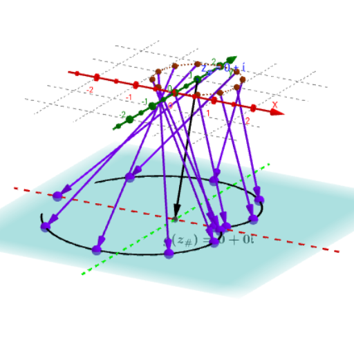
This example demonstrates mapping diagrams for functions with complex parameters, particularly focusing on circles. It involves core concepts in complex analysis such as mapping, parameter transformations, and loci. Using GeoGebra commands like Sequence, Circle, Point, etc., users can dynamically explore the impact of complex parameters on function graphs. Suitable for high school and above students or teachers for teaching and learning the geometric properties of complex functions.

GeoGebra Commands & Parameters

Sequence(0, m) → M
Zip(((2 * π) * k / m), k, M) → t_*
Zip((δ * ℯ^((t * ί))) + z_#, t, t_*) → z_*
Circle(z_#, δ) → circ
Point(circ) → A
Zip(h(z), z, z_*) → hz_*
Zip((x(z), y(z), ht), z, hz_*) → hpt_*
Line(O, ZY1) → Yax
Line(O, ZX1) → Xax
Zip(Vector[A, B], A, z_*, B, hpt_*) → hvec1_*
Vector(z_#, Gz1_#) → vecg_#
Vector(z_#, Hz1_#) → vech_#
Locus(PtAG, A) → gLoc
Locus(PtAH, A) → hLoc
Textfield(G) → InputBox1
Textfield(H) → InputBox2
Zip(g(z), z, z_*) → gz_*
Zip((x(z), y(z), ht), z, gz_*) → gpt_*
Zip(Vector[A, B], A, z_*, B, gpt_*) → gvec1_*
Point(xAxis) → x_#
Locus(gx_#, x_#) → greal
Locus(hx_#, x_#) → hreal